STATIONARITY ESTIMATION OF THE UK LABOUR FORCE: 1971-2010

JEO LEE¹*
¹Centre for Applied Research in Banking Finance, and Financial Regulation, Isle of Man International Business School, Douglas, Isle of Man, British Isles IM2 1QB
* Corresponding Author : j.lee@ibs.ac.im

Received : 21-01-2011     Accepted : 10-05-2011     Published : 16-05-2011
Volume : 2     Issue : 1       Pages : 57 - 78
Int J Econ Bus Model 2.1 (2011):57-78

Conflict of Interest : None declared

The instability and volatility of labour force participation in the United Kingdom over the last 39 years is examined. It is based on data obtained from the Labour Force Survey by the Office for National Statistics, at a disaggregated level, for males, ages 16 to 64, and females, ages 16 to 59, separately. Throughout four decades, the volatility of female employment levels is twice that of male employment. In contrast, the volatility in job growth appears to be minimal and similar in both men and women. Applying the unit root tests, cointegration, error-correction-model, and volatility model on the employment series, four main findings are suggested. First, the employment level appears to be mean-diverting, while the job growth appears to be mean-reverting. Second, the job growth reconfirms the mean-reversion in its volatility and the volatility clustering exists in it. Third, the level of employment and job growth in the male work force shows Granger causality on the female job growth and the level of employment. Last, the production and stock market levels might not be directly attributable to the levels of employment; perhaps other new jobs in the services industries like retail and health are more of an influencing factor.

Vector-error-correction model, ARCH model, cointegration, structural change, mean reversion, stationarity, volatility.

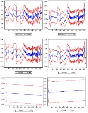
This study seeks to identify the stability and volatility in levels and growth of employment, in particular in the male and female workforce in the UK, utilising the Labour Force Survey (LFS) data from the Office for National Statistics (ONS). The ability to forecast levels of male and female employment is then discussed. The main assumption in this study is derived from the long-term trend that labour markets have no tendency to mean-reverting, owing to the development of technology and dynamic globalisation since the 1980’s though the major challenges to both global and national industries were the first and second oil crises during the early 1970s and 1980s [Fig-1] . In most developed countries, it is true that the number of jobs in manufacturing has declined while that in the service industry has risen since 1970. Many of the old jobs, including coal mining, the auto industry, textiles, and apparel manufacturing, have been replaced with sectors that include retail and wholesale services, information technology, health, education, and financial and business services that did not exist at the end of World War II. In particular, the largest percentage increase in job creation has been in government employment, information-processing, communications and managerial areas. This development provides a further hypothesis, an increased female workforce resulting from more widespread education and vocational training, together with a growth in service sectors.
Using the assumption stated above of mean diversion, a preliminary overview of each decade from 1971 to 2010 reveals that over that period, the volatility of female employment levels is higher than that of males. The volatility of female employment levels shows it is higher during the 1980s and for men in the 1990s [Table-1] & [Fig-1] . Job growth has been generally negatively skewed for each decade since 1971 - except recent period (2000-10) for male job growth [Table-2] . Since 1971, the volatility of workforce growth measured by standard deviation had been increasing for each decade. The level of female and male job growth is highest in the recent period (2000-2010), while the volatility of male job growth is high from 1980s onwards. For the female workforce over that period, the level of job growth has gradually increased up to the most recent period (1990s onwards). The proportion of non-working age job growth reveals a strikingly positive tendency over that period [Table-2] & [Fig-2] .
A unit root test was used in the longer term UK datasets to determine whether the level and growth in employment over time exhibited a mean-reverting behaviour, or not. If a series did not contain a unit root, the series was the stationary series that fluctuated around a constant long-run mean – this implied that the series, employment growth in this case, had a finite variance which did not depend on time: hence mean reversion. Next, the volatility of the level and growth of employment series was estimated using the volatility models based on the Generalised Auto Regressive Conditional Heteroscedasticity (GARCH). Finally, the Vector-Auto-Regressive (VAR) approach was used to find co-integration in the workforces over the economic cycle (using production and stock market indices).
Our empirical analysis suggests that the level of employment growth rates is mean-diverting. In addition, the ARCH effect in the employment growth series implies that the employment series has a volatility cluster—the deviation from the mean is not constant over time, and the deviation is smaller for some periods rather than others, and vice versa. The ARCH effect and unit root problem have serious consequences for forecasting and the forecast band could be narrower than the actual. Finally the co-integration of the level and growth of male and female employment in the UK reveals that the production and financial market – stock market in this case are rarely influenced by both over time.
The rest of the paper is as follows. In section 2 we discuss the methodology and data used for analysing workforce growth. Section 3 explains the results. The concluding remarks of the paper are given in section 4.

A comprehensive unit root method on the UK employment series (say, y_t) is used to test whether the series are stationary, hence mean reverting. A simple autoregressive of order one (AR (1)) process: y_t = ρ y_t-1 + where ρ is a parameter and to be estimated and the error term is assumed to be white noise ~ wn (0, σ²). After subtracting y_t-1 from both sides of the equation where α = ρ - 1, the standard Dickey-Fuller (DF) test by Dickey and Fuller (1979) has the null (H_o: α = 0, unit root) and alternative (H₁: < 0, stationary) hypothesis will be tested for all three cases; (i) random walk (), (ii) random walk with drift () and (iii) deterministic trend and a constant () using the Dickey-Fuller statistic (tau) statistic. Some of the alternative forms of unit root tests have been introduced, including the ADF (Augmented Dickey-Fuller, by Dickey and Fuller, 1981), an alternative to the ADF); the Phillips and Perron test (the PP test by Dickey Phillips and Perron, 1988); the KPSS test by Kwiatkowski, Phillips, Schmidt, and Shin (1992); the ERS test by Elliot, Rothenberg, and Stock (1996); and the NP test by Ng and Perron (2001). The ADF test offers a parametric correction for higher-order (AR (p) > AR (1)) correlation by assuming that y_t follows an AR(p) process where p is lag order. The null (H_o: ρ = 1, unit root) and alternative (H₁: |ρ| < 1, stationary) hypothesis will be tested using the test statistic where is the least square estimate and SE () is the usual standard error estimate. The PP test is a non-parametric test that is based on the statistic where is the estimate of the α and t_α is the t-ratio of the α, and SE () is coefficient’s standard error and S is the standard error of the test regression, is a consistent estimate of the error variance, and the term, f_o, is an estimator of the residual spectrum at zero frequency. The KPSS test must specify the set of exogenous regressors, x_t, and a method for estimating f_o.⁴ The critical value of the LM test statistic where f_o is an estimator of the residual spectrum at zero frequency. S(t) is a cumulative residual function: based on the residuals the regression of y_t on the exogenous variables x_t, a trend, and δ parameters to be estimated. The , error term, is assumed to be white noise. The ADF and PP tests however cannot distinguish a highly persistent stationary process from non-stationary process hence the power of unit root tests diminishes with a constant and a linear time trend in the test regression than those tests that only include a constant in the test regression (Schwert, 1989; Maddala and Kim, 2003). The ERS test is based on the quasi-differencing regression defined in a quasi-difference of y_t as d(y_t / a) that depends on the value ‘a’ representing the specific point alternative against which we wish to test the null y_t, if t = 1 otherwise y_t - αy_t-1, if t > 1; the a = where the de-trend data, , using the estimates associated with the , where the set of exogenous x_t, a constant or a constant and a linear time trend. A method for estimating f_o an estimate of the residual spectrum at zero frequency where the residuals are defined as . The NP unit root tests require a specification of x_t and a choice of method for estimating f_o and the statistics are modified forms of Phillips and Perron (1988) Z_α and Z_t statistics based upon the generalised-least-square de-trended data .
With the varied models of unit root tests have offered comparison for the performance. For instance, Nelson and Plosser (1982) applied the ADF test on the 14 U.S. macroeconomic series including employment. They used annual datasets for the time periods 1909-1970 and concluded that employment series is mean-diverting hence unit root exists in the series. Using the same dataset in Nelson-Plosser, Zivot and Andrews (1992) suggested a unit root test with endogenous break and drew the same conclusion as Nelson-Plosser that employment is mean-diverting. On the contrary, Zivot and Perron (1989) concluded that employment is mean-reverting subject to a structural break for the 1929 crash using the same dataset in Nelson-Plosser. The mixed results drown from the same data series indicate that unit root tests may not be reliable in the cases when a break point exists and did not include in the test regression or a break point does not exist and did include in the test regression, or the use of incorrect break date in the test regression.
We apply the ADF, the PP, the KPSS, the ERS, and the NP test on the employment level and growth are tested whether the series is mean-reverting subject to a structural change with a modified version: D*T_t is 0 if t < break duration, or 1, if t ≥ break duration.⁵ The results are reported below in Table 3 and Table 4 for the structural break model.

The volatility property in the level and growth of employment series is initially addressed in standard deviation [Table-1] and the instability ratio [Fig-1] for each decade. Based on standard deviation and instability ratios, which decade has higher employment volatility, higher standard deviation and higher instability ratio (sample variance divided by the mean) is evaluated. On the longer-term volatility in the employment series (1971-2010), it may be helpful to consider whether an explanation of volatility can be reasonably associated with empirical evidence from the employment series by applying volatility model that can describe the distribution of most financial data in which displays thicker tails.
ARCH effects have generally been found to be highly significant in financial markets of developed countries. The Autoregressive Conditional Heteroskedasticity (ARCH) type model (Engle, 1982) is considered to reflect the fact that economic agents and policy makers seem more sensitive to negative changes in employment level and growth. The various extensions of the ARCH model in particular the Generalized ARCH (GARCH) type models which has the same features of ARCH (q) model⁶. The major contribution of ARCH models allowed the conditional variance change over time as a function of past squared errors that captures the volatility clustering in asset return-the underlying forecast variance may change over time and is predicted by past forecast errors. GARCH (p,q) process is specified as a linear combination of past sample variance and the lagged conditional variance. In the GARCH model, the conditional variance is a function of past “squared” residual, and, hence, the sign of residual plays no role in affecting the volatility. GARCH models are the symmetric responses in the conditional variance to positive and negative changes in the series.⁷ The Exponential GARCH (EGARCH) model assumes that both the magnitude and the sign of the residual affect the volatility and it can accommodate not only “volatility clustering” but also “leverage effect” phenomena existing in most financial and monetary data and the model. We compare the magnitude of asymmetry in the UK employment measured for the male and female workforce.
The specification of the ARCH model incorporates squared conditional variance terms as additional explanatory variables that allow the conditional variance to follow an ARMA process with the residual: where is written as h_t and v_t has a zero mean and variance of one. The conditional variance can be defined as in a GARCH (p,q) process. Compared to the ARCH model, the GARCH model incorporates much of the information with large numbers of lags. To examine the volatility and asymmetry of volatility in the employment series, the EGARCH model is employed as the non-negativity constraint and does not need to be imposed and the asymmetries are also allowed for using an EGARCH (1, 1) model:



The empirical evidence from models used to forecast volatility suggest that negative shocks increase volatility more than positive shocks of the same magnitude. The empirical evidence also suggest that the magnitude of the asymmetric relationship between shocks and volatility may differ between males and females from the aspects in gender difference rooted from the social and industrial development over the period 1971-2010.

The stationary and instability in the level and growth of employment are examined above in where the level of employment is found to be non-stationary. The property of cointegration states that non-stationary variables have a strong tendency of the occurrence of cointegration. Applying cointegration, whether a long run relationship between variables even though the series are non-stationary, the combination of the two or three variables might be stationary hence an integration of first order I(1) where there is a long-term relationship between the series over 1971-2010 is assessed.⁸ There are various methods of cointegration tests such as the Engle-Granger cointegration test, cointegration regression - Durbin Watson and Johansen’s cointegration test. The Johansen’s cointegration - an autoregressive model is used in this paper: , where vector k from variable I(1) non-stationary, , and . To test for cointegration, the Johansen test defines that the trace test is applied to test for cointegration. The long-term relationship is explained in the matrix of several p variable when so that Ï€ consists of matrix Q and R with dimension (Ï€ = QR'), where matrix R is consists of r, 0, where , the largest i value of eigenvalue (k) the number of variables, T the number of observation, and r, the rank. If the counted value of LR is larger than the critical value of LR, cointegration for several variables exists. The maximum eigenvalue statistic,. . It proceeds first testing the null hypothesis of no cointegration against the alternative hypothesis of a full rank, i.e. all the series in the VAR system are stationary. Then, it tests the null hypothesis of one cointegrating relationship against the alternative of full rank and so on. The likelihood ratio statistics is sensitive to the presence of an intercept and trend, both in the series and in the cointegrating relationship. For short-term adjustment in the co-integration model, the Error Correction Model (ECM) in which the adjustment to correcting a disequilibrium can be written with the difference value (EC_t) as which is disequilibrium error. Engle and Granger (1987) and Johansen (1995) derives the test from the ECM structure of a Vector Autoregressive (VAR) system in which the variables include non stationary. This method simply consists of testing the restrictions imposed by cointegration on an unrestricted VAR. As expressed in Juselius (2006) the presence of unit roots in an unrestricted VAR corresponds to impose a reduced rank (rt = Г₁ Δy_t-1 + Пy_t-1 + μ + ε_t. If y_t ~ I(1) then Δy_t ~ I(0) then the matrix П cannot have full rank. This is because given the ECM, each equation of the VAR system would define a stationary variable Δy_t to be equal to a set of lagged stationary variables Г₁ Δy_t-1, a non stationary variable y_t-1 and a stationary error term ε_t, when EC_t equal to zero, y and x are in equilibrium condition. As y and x are rarely in an equilibrium condition, only the short-term relationship includes the first order lags of y and x are observe: ; 0 < Ø < 1. In this form, the value of y needs some time to adjust entirely towards the variation of x. According to Engle-Granger method, if two variables y_it and y_jt are non-stationary but cointegrated, the relationship between the two variables can be described using ECM that can be written as: where the term can be interpreted as a disequilibrium error from the previous time period (t - 1). , short-term influence, and long-term influence.
The unrestricted VAR method is applied to investigate the interdependencies in the variables, as a by-rproduct, a Granger causality based on the VAR system with each two and four time lags are tested. Assuming the series are stationary, the case of two stationary variables y_i,t and y_j,t in a VAR model in which _yit and _yjt are uncorrelated white-noise error terms. This can be expressed in matrix form:



where



The null hypothesis , and alternative hypothesis provide a test of whether a variable can be treated as exogenous in the VAR.

The Labour Forces Survey (LFS) data by the Office of National Statistics (ONS) are used to examine a longer-run analysis on the stability and volatility on UK employment over the period 1971 to 2010. The raw data are rolling monthly quarterly frequency for men 16 to 64 and women 16 to 59. The data begin with 1971:Q1 (quarterly data series) and ends with 2010:Q3. Other information used are the production index and stock index from the IMF to determine whether production or the financial sector (stock market, in this case) would influence the level and growth of employment in the long run.
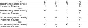
Both the entire sample period and each decade are examined for the level and job growth of male and female workforces, whether all data share the same statistical moments — mean, standard deviation and instability ratio — or not. To establish the time-variant pattern, the data series are divided into four decades (1971-79, 1980-89, 1990-99 and 2000-10:Q3); the first and fourth are not complete decades because of data availability. Instead of using decades, it might be meaningful to divide the data according to economic or business cycles; however, the duration of each cycle varies, and there have been less-obvious shocks to the cycle that the time span might infuse with an exaggerated significance. [Fig-1] illustrates the level and growth of male and female employment, industrial production and stock price movements for 1971-2010. It shows a similar upward trend in the level of female employment, production and stock prices while the level of male employment depicts a different pattern – two deep downturns around the shocks in the 1970s and 1980s. Descriptive statistics are presented in [Table-1.1] and [Table-1.2] . In [Table-1.1] , the average level of male (14,581) and female workforces (10,747) shows that there are 26 percent more males, while the volatility in the female workforce (1,331) is much higher than the male’s (559). The table indicates a tendency for the level of male and female employment to decrease, hence a negative-skewness. The job growth of both workforces shows marginally positive-skewness, with a higher rate for women (0.31) than men (0.11). The Jarque-Bera test suggests that returns are normally distributed at the 10 percent level of significance based on the sample kurtosis and skewness. For each decade, [Table-1.2] suggests that the highest volatility measured with standard deviation for the level of female and male employment is during the 1980s (587) and 1990s (402). The gap in volatility has been narrowed for the most recent period (2000-10). Each decade shows higher volatility when compared to the 1970s. Similarly, an instability ratio measured by the ratio based on the variance divided by the mean values is illustrated in [Fig-2] . The highest ratio of instability in the female workforce was in the 1980s; and the level of male employment is highest during the latest sub-sample period according to the instability ratio, while it is highest during the 1990s based on the standard deviation, as in [Table-1.2] . This indicates that instability in the level of the male workforce is highest during the latest decade. Interestingly, [Fig-3] illustrates a gradual increasing tendency in non-working age employment (men over 65; women over 59) since the 1990s. This probably reflects demographic changes for the four decades, which likely will continue with extended life expectancy and evolution of a knowledge-based services industry [Fig-4] . The descriptive statistics for UK job growth from 1971Q1 to 2010Q3 are based on the ratio of the gap between two consecutive periods for female (age 16 to 59) and male (16 to 64) workforces and are summarised in [Table-1.3] . Job growth for each decade since 1971 has shown a negative-skewness except for males in the 2000 - 2010. For each decade, the volatility of job growth is similar for both sexes. Overall, it clearly indicates that job growth in both workforces has been improved only marginally (males, 0.0000; females, -0.0008), and volatility in job growth is similar (males, 0.0017; females, 0.0016) for the whole period.

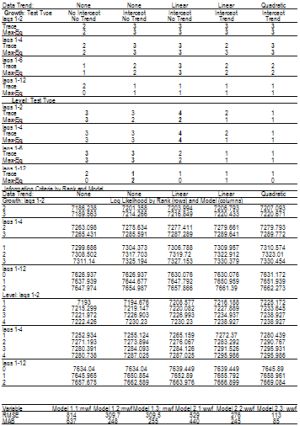
[Table-1] shows that the level of female employment has higher volatility than male employment while job growth for males is higher in volatility than that for females. [Table-2] shows results of unit root tests of ‘mean reversion,’ whether the level and growth in employment eventually move back towards the historical average or not. Two types of unit root tests, (i) intercept and (ii) a constant and a linear trend, were considered with the test options; on the level and first differenced were used. The null hypothesis is an existence of unit root, and the alternative is stationary; hence, if the test statistics can reject the null hypothesis, the series would be mean-reverting.
The results of five unit root tests -- ADF, PP, KPSS, ERS and Ng-Perron -- for the level of employment for men and women are consistent, exposing evidence of non-stationarity on the employment level when incorporating a constant or drift parameter in the test regression, hence mean-diversion in the level of employment. Once first differenced, the level of employment series, all tests agreed that the series are stationary, hence mean-reverting. An exceptional case is in the Ng-Perron test results on the first differenced series. These results contradict the results when the regression equation has an intercept but without trend term from the results based on the ADF, PP and KPSS at 1 percent significance level; however, the null of unit root can be rejected at the 10 percent level of significance.
The unit root results on the growth of employment from all unit root tests with two test options, intercept and constant and trend on the level and first differenced employment growth series, reject the null hypothesis; hence, the growth of employment has the same conclusion, i.e., that the growth series are mean reverting. Both ERS and Ng-Perron tests for the growth of employment using the level of the series indicate that the series is weakly stationary when including an intercept term in the equations. For example, the results based on Ng-Perron and the ERS tests cannot reject the null at the 1 percent significance for the level of employment growth in the regression equation with a constant but without a trend term. In the case of the result from the Ng-Peron test, the first differenced growth of female employment cannot reject the null of non-stationarity. Although the Ng-Perron unit root test has a confusing conclusion, if we set the level of significance at 10 percent then the null hypothesis of a unit root can be rejected. In sum, all unit root tests are consistent with the results that the level of employment contains a unit root; hence, a ‘mean-diversion.’ On the other hand, the job growth of employment is found to be a mean-reversion; hence, stationary.⁹

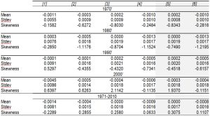
We have found that the level of employment growth series is non-stationary and mean-diverting, which implies that the mean and variance from the level of employments series are not consistent over time and may be time dependent. The time invariant property in the long term employment series is examined using a simple form of structural break and the ARCH effect. Whether there is any change in a trend characteristic in the series over time: y_t = β_o + β₁ T_t + β₂ T2_t + ε_t where y_t is a dependent variable, time variable (T) is a time dummy t= 1,2,…..T. To capture the non-linearity of the trend, we also include time-square (T2). [Table-3] shows results of the trend estimates together with the Akaike information criterion and Durbin-Watson statistics. The growth of employment for male and female workforces and the level of male employment show that β₁ and β₂ are statistically insignificant. For the level of male and female employment, the series follows a linear trend, the β₁ coefficients are all statistically significant, and the sign of the β₁ coefficients indicate increasing trends. [Table-3] also shows the estimates of the ARCH effect in the level and growth series. The specification of models varies depending on inclusion of the trend dummy with or without the ARCH term (AR 1 to 3) in the equation: y_t = C + T + Log(y_t-1) + AR (1 to 3) + ε_t where y_t is set Log(y_t) for the level and y_t for the growth of employment. The results conclude the existence of the ARCH effect in all series. In particular, the model including AR(1) term shows sufficient effect on the level and growth of employment, although lagged AR (2) and AR (3) are also significant statistically but with marginal size in the coefficients.
[Table-4] reports the results with different specification of models to estimate structural breaks for the level (Models 1, 3, and 5) and the growth (Models 2, 4, and 6) of the employment series:
Model 1: LOG(level)=C(1)+C(2)*T+C(3)*DOS2+C(4)*DOS2*T+[ AR(1)=C(5) ]
Model 2: Growth=C(1)+C(2)*T+C(3)*DOS2+C(4)*DOS2*T+[ AR(1)=C(5) ]
Model 3:
Log (level)=C(1)+C(2)*T+ C(3)*D1+ C(4)*D2+ C(5)*D3+ C(6)*D4
Model 4:
Growth = C(1)+C(2)*T+ C(3)*D1+ C(4)*D2+ C(5)*D3+ C(6)*D4
Model5:
Log (level)=C(1)+C(2)*T+ C(3)*D1+ C(4)*D2+C(5)*D3+C(6)* 4+C(7) *IP+C(8)*SP
Model 6:
Growth =C(1)+C(2)*T+ C(3)*D1+ C(4)*D2+ C(5)*D3+C(6)*D4+C(7)* IP+C(8)*SP.
In Models 1 and 2, DOS2 indicates the oil shock dummy set 1973Q3: DOS2=1*(DOS1=0)+0*(DOS1=1),s where DOS1=1(t<=1973Q3)+0*(t>1973Q3); and where AR (1) autoregressive with lag 1. In Models 3-6, D, IP and SP, these indicates structural duration dummy, industrial production, and stock market proxy. Modes 1 and 2 utilize a dummy variable of 1973Q3 where an oil shock break point was set to estimate a step-wise structural break for both the level (Model 1) and the growth (Model 2) of employment for male and female workforces. The estimates of Model 1 suggest that the coefficients of trend, the ARCH effect are statistically significant in the level of female employment, while the coefficients of trend and structural break point and the oil shock are statistically significant for the level of male employment. Model 1, therefore, suggests that the level of male employment is more sensitive to the shock. All coefficients of Model 2 on the growth of employment for males and females are statistically insignificant except the joint effect from the oil shock and trend. This again indicates that job growth is stationary over the time. In Models 3 and 4, instead of inclusion of structural break points, duration of structural breaks is used. For instance, D1, D2, D3 and D4 denote 1973 September (oil shock and stock market crash in the UK, 1973-75); 1983 September (the second oil shock and recession, 1981 – 1983); 1992 September (black Wednesday stock market crash); and 2008 September (the crises of Russia, automotive industry and subprime). [Table-4] reports the results based on the specifications with the duration of each structural break without (Models 3 and 4) and with industrial production (IP) and stock market (SP) series (Models 5 and 6). The estimates from Model 3 on the level suggest that the latest shock is statistically significant to the level of female employment, in which the shock decreased the level of the series, while all shocks on the level of male employment are statistically significant with negative impact from the second oil shock and the 1992 market crash. Both the second oil shock and the latest 2008 shock are statistically significant to the job growth in male and female employment, while the 1992 shock is also statically significant to the growth of male employment. The job growth for males and females for the entire period is still stable regardless of the shocks. Models 5 and 6 include two additional variables: industrial production (real factor) and stock market (financial factor) in addition to the shock variables (D1 – D4). The results suggest that both production and the stock market are statically significant; however, the size of the coefficients suggests that the magnitude is marginal -- less than 10 percent on the employment level and less than 1 percent to job growth. Interestingly, the production and stock market evolution for the decades has had a negative impact on job growth and the level of male employment (see [Fig-4] ). In this specification, only the second oil shock is revealed statistically significant on the level of employment while the recent shock is statistically more significant in job growth for men and women.

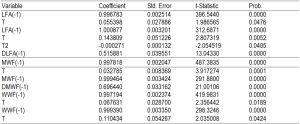
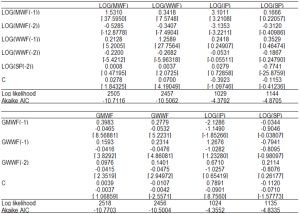
The implication of the ARCH effects is that the employment growth series has a volatility cluster-some periods are more volatile than others (see Tables 1 and 3, Fig. 2), hence the variance is not constant over time and has high variance for some periods than others. That also implies, the forecast band, upper and lower band of the forecast, will not be constant and may be smaller for some time period than others, and vice versa. To estimate volatility in the longer-term employment series (1971-2010), the EGARCH model is used. The estimates of the univariate and unrestricted EGARCH model (1,1) restrict the coefficients of production and stock market measuring volatility spillovers to be zero for the former, are presented in [Table-5] . The parameter we are initially interested in is the C(2) and C(7) asymmetric coefficient. The level of male workforce and the growth of female workforce have the expected sign in the restricted EGARCH model that bad news would have more impact on the level of male employment and the job growth for female workforce. The job growth of male workforce shows positive sign that good news would more impact on bad news to the job growth for man. From the estimates in the unrestricted EGARCH model, the asymmetric coefficient of the level of male workforce and the job growth for woman show negative signs though they are not statistically significant. The coefficient of the job growth of male workforce is statistically significant, however, the positive sign indicates that positive shocks generate more volatility than negative shocks for job growth for men. The volatility persistence parameters C(4) and C(8) are all positive and significant for both the level and job growth of the male and female employment in two EGARCH models indicating that a shock to the conditional variance is persistent. The parameter is close to 1 in job growth (0.995 and 0.999; 0.99 and 0.99 for woman and man respectively) and level of employment (0.87 and 0.83; 0.91 and 0.87 for woman and man respectively) in two EGARCH models.¹² The positive values of the parameter (C4), the presence of volatility clustering, are all statistically significant at the 10% level for both male and female employment level and job growth suggesting that large changes in level and growth of employment are more likely to be followed by a large change in the level and growth of either sign than by small change in the level and growth of employment. [Table-6.2] , the size of coefficients of the previous value of production and stock market on the level and the growth of men and women is almost zero or statistically insignificant except the coefficient of production on the level of employment for females that is statistically significant, again the size is small (0.0001).

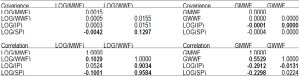
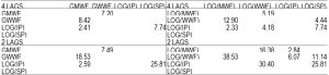
The Johansen approach for multiple equations uses the four variable Vector Autoregressive (VAR) system: z_t={y_t,wwf; y_t,mwf; IP_t; SP_t} where yt can be the level or the growth of employment. zt in a vector error-correction model contains 4 x 4 matrix which would contain the long-run relationships. In this VAR specification for z_t, the coefficients of the covariance and correlation are reported in [Table-7] . First, the summary of the estimates of covariance shows statistically insignificant except the case between job growth of females and the stock price is positive (0.13). Second, the correlation coefficients are all negative between job growth of male (-0.29) and industrial production; and females (-0.01) to industrial production; and between the stock price and the male job growth (-0.23), in contrast, a positive correlation coefficients are found between production (0.90) and stock price (0.96). Lastly, the Granger causality based on the VAR rejects the null hypothesis of no causation at least 5% level of significance that the level and growth of male employment are revealed to which causes the woman’s employment level and its job growth. The stock market causes the level and growth in woman’s employment. The size of coefficients of Causality test with two time lags is revealed to be larger than when the time interval with 4 lags. [Table-8] presents the results of causality based on the equation in Section 3.4 with 2 and 4 time lags as a by-product of the VAR system. The findings indicate that the job growth of the male work force causes the job growth of the female work force (8.42 and 18.53 for 4 and 2 lags respectively) while the opposite appears much lower (7.2 and 7.49 for 4 and 2 lags respectively). The production and stock markets cause no change to job growth. The level of male employment influences the female employment level (12.9 and 38.5 for 4 and 2 lags respectively) while the opposite causation made is (5.19 and 16.38 for 4 and 2 lags respectively). The production cause only a short lag positive impact (2.84 and 6.07 for 2 lags for men and women respectively) while the causation from the stock market appears only on the level of female employment (4.44 and 11.14 for 2 and 4 time lags respectively). [Table-9] reports the number of cointegrating relations that are the results of Johansen cointegration tests based on the trace statistics (λ_trace) and maximal-eigenvalue statistic (λ_max) across four variables. The Johansen method is known to be sensitive to the lag length (see Banerjee et al., 1993). Different lag length of order (lags 1-2; lags 1-4; and lags 1-6; and lags 1-12) is used for the VAR system comprising the four variables for various lag lengths and calculate the respective Akaike Information criterion (AIC) in order to determine the appropriate lag length for the cointegration test for the same sample period 1971Q1 – 2010Q3. Different test types (Model 1: no-intercept with no-trend; Model 2: intercept with no-trend; and Model 3: intercept and trend) are also specified. First, for the level of employment, once the series is first differenced, the optimal model based on the AIC and the log-likelihood (LL) is found to be the ‘intercept with no-trend (up to 4 lags)’ which shows a full rank (πz _t-1, z_t-1, and ut are I(0)) that all the variables in z_t are stationary. When the specification is set up to 12 lags, only one cointegrating relationship across the variables is found. Second, for the growth of employment, there are three cointegrating relations with the Model 2 and Model 3 up to 4 lag length are both. However, when lag length of order 12 only one cointegrating relationship is shown at most. In all equations the diagnostics suggest that the residuals are Gaussian. The estimated equations based on the vector error correction model (VECM) discussed in Section 2.3 are as follow:

[1] D(LOG(MWF)) =
0.0009*(LOG(MWF(-1)) - 2.406*LOG(WWF(-1)) + 3.130*LOG(IP(-1)) - 0.0102*LOG(SP(-1)) - 1.2213) + 0.3951*D(LOG(MWF(-1))) + 0.2286*D(LOG(MWF(-2))) + 0.1535*D(LOG(WWF(-1))) + 0.0862*D(LOG(WWF(-2))) - 0.0006*D(LOG(IP(-1))) - 0.0025*D(LOG(IP(-2))) - 0.0021*D(LOG(SP(-1))) + 0.0028*D(LOG(SP(-2))) - 0.0002

[2] D(LOG(WWF)) =
- 0.0005*(LOG(MWF(-1)) - 2.406*LOG(WWF(-1)) + 3.1298*LOG(IP(-1)) - 0.0102*LOG(SP(-1)) - 1.223) + 0.257*D(LOG(MWF(-1))) + 0.0698*D(LOG(MWF(-2))) + 0.2591*D(LOG(WWF(-1))) + 0.1595*D(LOG(WWF(-2))) + 0.0027*D(LOG(IP(-1))) + 0.0019*D(LOG(IP(-2))) - 0.0053*D(LOG(SP(-1))) + 0.0043*D(LOG(SP(-2))) + 0.0005

[3] D(GMWF) =
- 0.2055*(GMWF(-1) - 1.1989*GWWF(-1) + 0.0078*LOG(IP(-1)) - 0.0004*LOG(SP(-1)) - 0.0345) - 0.3602*D(GMWF(-1)) - 0.1084*D(GMWF(-2)) - 0.0705*D(GWWF(-1)) + 0.0469*D(GWWF(-2)) + 0.0014*D(LOG(IP(-1))) + 0.0006*D(LOG(IP(-2))) + 0.0012*D(LOG(SP(-1))) - 0.0039*D(LOG(SP(-2))) + 1.638e-05

[4] D(GWWF) =
0.482*( GMWF(-1) - 1.1989*GWWF(-1) + 0.0078*LOG(IP(-1)) - 0.0004*LOG(SP(-1)) - 0.0345) - 0.1693*D(GMWF(-1)) - 0.0324*D(GMWF(-2)) - 0.174*D(GWWF(-1)) - 0.0152*D(GWWF(-2)) - 0.0019*D(LOG(IP(-1))) - 0.0031*D(LOG(IP(-2))) + 0.0024*D(LOG(SP(-1))) - 0.003*D(LOG(SP(-2))) + 6.99e-06

The VECM [1] - [4] are based on that could be stated as first order ECM with , where α₁, short-term coefficient, α₂, error correction component, β₁, long-term coefficient. The cointegrating coefficient in the long run model (ecm_t-1) is -0.206 (GMWF(-1)); 0.048 (GWWF(-1)); 0.0009 (MWF(-1)); and -0.0005 (WWF(-1)) to the change in male (DGMWF) and female (DGWWF) job growth; male (DMWF) and female (DWWF) employment respectively. To restore the stability of the level of male employment in Model [1] , the previous level of female employment needs to be lowered (-2.41) with higher previous industrial production (3.13); in Model [2] , the current stability of the level of female employment would be achieved with lower previous own level of employment (-2.41) with higher previous production (3.13); in Models [3] and [4] , the current stability of both male and female job growth would be achieved with lower previous job growth of the female work force (-1.20). The insignificance of the ECM component for the production and stock market variables in addition to the insignificance from the short run equation (in VAR) suggest that the two variables are weakly exogenous to the model both In the long- and short-run models in the VECM.

The main findings first indicate that the level of male employment is much too difficult to forecast than that of the female employment level. Second, forecasting the job growth for both males and females show similar forecasting error. Lastly, production and stock market help marginally to forecast for the job growth for males and females, and the level of male employment. [Fig-5.1] and [Fig-5.2] illustrate the long-run forecasting performance for the period of 1971Q1-2015Q3 based on the actual observations for the level of employment for males and females (WWFF). For the estimation, the White heteroscedasticity consistent coefficient covariance is used, and the Root Mean Squared Error (RMSE) and the Mean Absolute Error (MAE) from Models 1 and 2 are reported with Figures 5.1-5.2. Comparing the RMSE and the MAB, the optimal foresting model for the level of male employment is Model 1.2 that has only its own lagged variable and the employment level of females. In contrast, the Model 2.3 is the optimal forecasting model for the employment level of women which includes own previous value, the level of male employment and its lagged value, production and its lagged value, and stock market and its lagged value. The main results from forecasting the level of employment with 2 suggest that production and stock market job would not useful for the forecasting of male employment. The performance of the long-run foresting for the job growth during 19171Q1 – 2015Q3 is illustrated in [Fig-5.2] with the RMSE and the MAB. The growth in employment for both males and females are similar (0.0017 – 0.0012 and 0.0016-0.0012 for the RMSE between Model 3.1 and 3.3; and between 4.1 and 4.3 respectively for male and female).

The instability and volatility of the UK labour market for the period from 1971 to 2010 was examined. The data used for this long-term analysis was based on the Labour Force Survey by the Office of National Statistics (the UK ONS), starting from 1Q1971 and end 3Q2010 on the employment levels and job growth for the male and female workforce (ages 16 to 64 and 16 to 59 respectively). Periodic characteristics for each decade reveal that there are significant differences in the shapes and patterns between the male and female employment levels. Throughout four decades, the female employment level is more than twice as volatile (1434) than that of the level of male employment (558). In particular, the highest volatility is found in the level of the female employment during the 1980’s. The volatility of male employment was the highest during 1990’s; however when measured by the instability ratio, the latest decade (2000’s) was the most volatile. Interestingly the volatility in the job growth appears to be similar in both males and females for the same period.
The results based on the stationary test suggest that the employment level appears to be mean-diverting and the job growth appears to be mean-reverting. The estimates from the EGARCH model reconfirm that the mean-reversion of volatility in job growth as shown in the volatility clustering parameter on job growth is close to 1. The evidence based on the ECM also suggests that the previously lower female job growth would restore the next period’s equilibrium level to both male and female job growth. Moreover, previous lower female employment levels and higher production would restore the level of males and females employment for the next period. Besides, according to the volatility model, the level of male employment reacts more to bad news than good news, on the other hand good news affects the volatility of male job growth. The results from the Johansen cointegration based on a VAR system indicates that the level and job growth in male and female employment are interlinked with production and stock market over the four decades. The evidence from cointegration and causality, however, it suggests that the production and stock market have little influence on the job growth and only marginally relate to the level of employment for the male work force.
In summary, the empirical analysis suggests that the level of employment is mean-diverting in that the ‘root mean squared error’ and the ‘mean absolute error’ in forecasting is wider in the level of male employment and the evidence of difficulty to forecast for the male employment level into the future. In contrast, the standard error of forecasting job growth reveals to be narrow to both male and female job growth so that there is evidence of a mean-reversing property in the job growth. The policy implications from the main findings suggest that the old jobs might be replaced with new jobs; hence there is mean-diversion in the labour market. In addition, there are other sectors that have evolved over the four decades such as the services sectors including retail, health, and technology. Therefore, production and financial market changes might not directly attributable to the levels of employment. The job growth would be stationary to that mean reverting. This study also identified the historically known crashes and crises those are statistically significant; however, the job growth is revealed to be strikingly stable throughout the decades. Measuring the different types of shocks, less-obvious-shocks and unknown-risks on the level of employment remains for further study.

[1] Bai J. (1998) Econometric Theory, vol. 14(05), 663-669.  
» CrossRef   » Google Scholar   » PubMed   » DOAJ   » CAS   » Scopus  

[2] Baillie and Bollerslev T. (1989) Journal of Business and Economic Statistics 7, 297-305.  
» CrossRef   » Google Scholar   » PubMed   » DOAJ   » CAS   » Scopus  

[3] Baillie and Degenerate R. P. (1989) Journal of Financial Service Research 3, 55-76.  
» CrossRef   » Google Scholar   » PubMed   » DOAJ   » CAS   » Scopus  

[4] Banerjee A., Lumsdaine R. and Stock J. (1992) Journal of Business Economics and Statistics, 10, 271-287.  
» CrossRef   » Google Scholar   » PubMed   » DOAJ   » CAS   » Scopus  

[5] Banerjee A., Dolado J.J., J.W. Galbraith and Hendry D.F. (1993) Cointegration, Error-Correction and the Econometric Analysis of Non-Stationary Data. Oxford: Oxford University Press.  
» CrossRef   » Google Scholar   » PubMed   » DOAJ   » CAS   » Scopus  

[6] Berman E., Bound J. and Machin S. (1998) Journal of Economics, 113, 1245-79.  
» CrossRef   » Google Scholar   » PubMed   » DOAJ   » CAS   » Scopus  

[7] Desai T., Gregg P. Steer J. and Wadsworth J. (1999) Gender and the Labour Market in P. Gregg and J. Wadsworth (eds.) The State of Working Britain, Manchester: Manchester University Press.  
» CrossRef   » Google Scholar   » PubMed   » DOAJ   » CAS   » Scopus  

[8] Black F. (1976) Studies of stock price volatility changes, American Statistical Association, 177-181.  
» CrossRef   » Google Scholar   » PubMed   » DOAJ   » CAS   » Scopus  

[9] Bollerslev T. (1986) Journal of Econometrics, 31, 307-327.  
» CrossRef   » Google Scholar   » PubMed   » DOAJ   » CAS   » Scopus  

[10] Boothe P. and Glassman D. (1987) Journal of International Economics, 22, 297-319.  
» CrossRef   » Google Scholar   » PubMed   » DOAJ   » CAS   » Scopus  

[11] Caner M. and Kilian L. (2001) Journal of International Money and Finance, vol. 20(5), 639-657.  
» CrossRef   » Google Scholar   » PubMed   » DOAJ   » CAS   » Scopus  

[12] Christiano L. (1992) Journal of Business Economics and Statistics, 10, 237-250.  
» CrossRef   » Google Scholar   » PubMed   » DOAJ   » CAS   » Scopus  

[13] Christie (1982) Journal of Financial Economics. 10, 407-432.  
» CrossRef   » Google Scholar   » PubMed   » DOAJ   » CAS   » Scopus  

[14] Clemente J., Montanes A., and Reyes M. (1998) Economics Letters, 59(2), 175-182.  
» CrossRef   » Google Scholar   » PubMed   » DOAJ   » CAS   » Scopus  

[15] Cutler J. and Turnbull K. (2001) A disaggregaed approach to modelling UK labour force participation, Discussion paper No. 4, Bank of England.  
» CrossRef   » Google Scholar   » PubMed   » DOAJ   » CAS   » Scopus  

[16] De Jong, Kemna F. A., and Kloek T. (1990) The impact of option expirations on the Dutch stock market”, Erasmus University, Rotterdam.  
» CrossRef   » Google Scholar   » PubMed   » DOAJ   » CAS   » Scopus  

[17] Dickey D. and Fuller W. (1979) Journal of the American Statistical Association, 74, 427-431.  
» CrossRef   » Google Scholar   » PubMed   » DOAJ   » CAS   » Scopus  

[18] Dickey D. and Fuller W. (1981) Econometrica, 49, 1057-1072.  
» CrossRef   » Google Scholar   » PubMed   » DOAJ   » CAS   » Scopus  

[19] Diebold F. X. (2007) Elements of Forecasting. 4^th ed., Thomson South-Western.  
» CrossRef   » Google Scholar   » PubMed   » DOAJ   » CAS   » Scopus  

[20] Elliott G., Rothenberg T. & Stock J (1996) Econometrica 64, 813—836.  
» CrossRef   » Google Scholar   » PubMed   » DOAJ   » CAS   » Scopus  

[21] Engle R. F. (1982) Econometrica, 50, 987-1008.  
» CrossRef   » Google Scholar   » PubMed   » DOAJ   » CAS   » Scopus  

[22] Engle R. F. and Bollerslev T. (1986) Econometric Reviews, 5, 1-50.  
» CrossRef   » Google Scholar   » PubMed   » DOAJ   » CAS   » Scopus  

[23] Fuller W. A. (1976) Introduction to Statistical Time Series. New York: John Wiley.  
» CrossRef   » Google Scholar   » PubMed   » DOAJ   » CAS   » Scopus  

[24] Gregg P. and Wadsworth J. (1999) Economic Inactivity in P. Gregg and J. Wadsworth eds. The State of Working Britain, Manchester: Manchester University Press.  
» CrossRef   » Google Scholar   » PubMed   » DOAJ   » CAS   » Scopus  

[25] Harberger A.C. (1993) The search for relevance in economics, American Economic Review papers and Proceedings, 83.116.  
» CrossRef   » Google Scholar   » PubMed   » DOAJ   » CAS   » Scopus  

[26] Hsieh (1989) Journal of Business & Economic Statistics, 7, 3.  
» CrossRef   » Google Scholar   » PubMed   » DOAJ   » CAS   » Scopus  

[27] Kim D. & Perron P. (2009) Journal of Econometrics, 148, 1–13.  
» CrossRef   » Google Scholar   » PubMed   » DOAJ   » CAS   » Scopus  

[28] Kwiatkowski D., Phillips P., Schmidt P. & Shin Y. (1992) Journal of Econometrics 54(1-3), 159-178.  
» CrossRef   » Google Scholar   » PubMed   » DOAJ   » CAS   » Scopus  

[29] Layard R., Nickell S.N. and Jackman R. (2005) Unemployment, macroeconomic performance and the labour market, Oxford University Press, 2 nd edition.  
» CrossRef   » Google Scholar   » PubMed   » DOAJ   » CAS   » Scopus  

[30] Lumsdaine R.L. and Papell D.H. (1997) Review of Economics and Statistics, 79, 212-218.  
» CrossRef   » Google Scholar   » PubMed   » DOAJ   » CAS   » Scopus  

[31] Maddala G. and Kim I. (2003) Unit Root, Cointegration, and Structural Changes. Cambridge University Press.  
» CrossRef   » Google Scholar   » PubMed   » DOAJ   » CAS   » Scopus  

[32] Nelson C. R. and Plosser C. I. (1982) Journal of Monetary Economics 10, 139–162.  
» CrossRef   » Google Scholar   » PubMed   » DOAJ   » CAS   » Scopus  

[33] Nelson D. B (1991) Econometrica, 59, 347-370.  
» CrossRef   » Google Scholar   » PubMed   » DOAJ   » CAS   » Scopus  

[34] Ng S. and Perron P. (2001) Econometrica 69, 1519–1554.  
» CrossRef   » Google Scholar   » PubMed   » DOAJ   » CAS   » Scopus  

[35] Nickell S. (1999) Unemployment in Britain in P. Gregg and J. Wadsworth, eds. The State of Working Britain, Manchester: Manchester University Press.  
» CrossRef   » Google Scholar   » PubMed   » DOAJ   » CAS   » Scopus  

[36] Nunes L.C., Kuan C-M. and Newbold P. (1997) Econometric Theory, 11, 736-49.  
» CrossRef   » Google Scholar   » PubMed   » DOAJ   » CAS   » Scopus  

[37] Papell D. H. and Prodan R. (2003). Restricted Structural Change and the Unit Root Hypothesis. Working paper, University of Houston.  
» CrossRef   » Google Scholar   » PubMed   » DOAJ   » CAS   » Scopus  

[38] Perron P. (1989) Econometrica, 57, 1361-1401.  
» CrossRef   » Google Scholar   » PubMed   » DOAJ   » CAS   » Scopus  

[39] Perron P. & Vogelsang T. (1992) Journal of Business and Economic Statistics, 10, 467-470.  
» CrossRef   » Google Scholar   » PubMed   » DOAJ   » CAS   » Scopus  

[40] Phillips, P. & Perron, P. (1988) Testing for a unit root in time series. Biometrika, 75, 1361-1401.  
» CrossRef   » Google Scholar   » PubMed   » DOAJ   » CAS   » Scopus  

[41] Schwert W. (1989) Journal of Business and economic Statistics, 7, 147-159.  
» CrossRef   » Google Scholar   » PubMed   » DOAJ   » CAS   » Scopus  

[42] Wood A. (1994) North-South Trade, Employment and Inequality, Oxford: Clarendon Press.  
» CrossRef   » Google Scholar   » PubMed   » DOAJ   » CAS   » Scopus  

[43] Zivot E. and Andrews D.W.K. (1992) Journal of Business and Economic Statistics, 10, 251-270.  
» CrossRef   » Google Scholar   » PubMed   » DOAJ   » CAS   » Scopus  

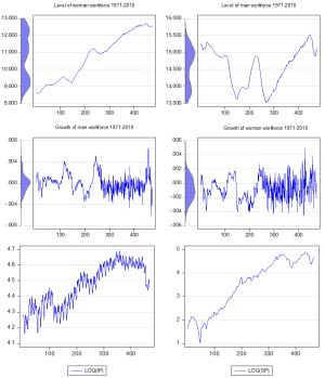	Fig. 1- Distribution and trend in the level & growth of employment: 1971Q1-2010Q3 Level of UK industrial production (IP) and Stock prices (SP): 1971Q1-2010Q3
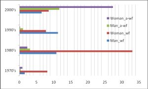	Fig. 2- Instability in UK employment level during 1971 – 2010 Notes: Instability is measured by the ratio between sample variance divided by the mean value. Man_wf, Man_a-wf, woman_wf, and woman_a-wf respectively indicates: Male workforces (age 16-64); Female workforces (age 16-59); Male all employment (16 over) and Female all (16 over).
	Fig. 3- Evolution of non-working age employment growth: 1971 – 2010
	Fig. 4- Workforce jobs by industry (1978-2010) Source: Dataset name is ons1 from Office for National Statistics. Notes: variables: Top-left-hand-side, Mining & Mnfg= sum of mining and quarrying and manufacturing jobs; Edu&Health=sum of education and human health and social work activities jobs; Infor & Fin=information, communication, financial and insurance jobs; Public sector jobs. Unit, thousands.
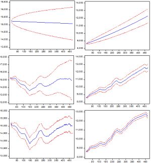	Fig. 5.1- Forecasting of the level in employment with 2 standard error: 1971-2015
	Fig. 5.2- Forecasting of the growth in employment with 2 standard error: 1971-2010
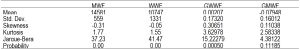	Table 1.1- Descriptive statistics of UK employment: 1971Q1-2010Q3 Notes: MWF, WWF, GWWF, and GMWF indicates the level of male work forces age between 16 and 64, the female work forces age between 16 and 59, the growth of female work forces 16 – 59 (x100), and the growth of male work forces 16 – 64 (x100) respectively. MWF and WWF, the observations used for MWF and WWF are 474, and GWF and GMWF are 473, respectively
	Table 1.2- Distribution of the level of UK employment for each decade Notes: [1] Male workforces (age 16-64); [2] Female workforces (age 16-59); [3]; Male all employment (16 and over) – male workforces (age 16-64); and [4] Female all employment (16 and over) – Female workforces (age 16-59).
	Table 1.3- Descriptive statistics of the job growth of UK for each decade Notes: [1] is the growth gap between all workforces and all workforces; [2] the growth of all workforces; [3] the growth of man age over 16; [4] the growth of woman age over 16; [5] the growth of man workforce age between 16 and 64; [6] the growth of woman workforces age between 16 and 59.
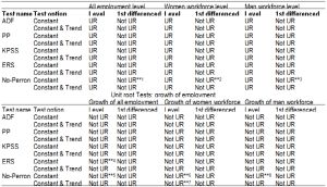	Table 2- Unit root tests on the level and growth of UK employment: 1971-2010 Unit root Tests : level of employment Notes: Critical values for KPSS, NP, ER, and ADF are shown in Kwiatkowski-Phillips-Schmidt-Shin (1992, Table 1), Ng-Perron (2001, Table 1), Elliott-Rothenberg-Stock (1996, Table 1), MacKinnon (1996) one-sided p-value. **1, Ng-Perron test statistics reject for MSB (0.1798) at 5% where NP other asymptotic critical values reject the null of Mza, MZt and MPT, **2, Ng-Perron test statistics reject for MSB (1.5503) at 5% (3.17) where NP other asymptotic critical values reject the null of Mza, MZt and MPT; **3, Ng-Perron test statistics reject for MSB (0.184) at 5% (0.233) only where NP other asymptotic critical values reject the null of MZa, MZt and MPT; **4, Elliott-Rothenberg-stock test statistic at 5% (3.26) can be rejected with the test statistics (2.19) but not at 1% (1.99); **5, Ng-Perron test statistics cannot reject the null for MPT(1.550) at all significance levels where NP test statistics reject other asymptotic critical values MZa, MZt and MSB, **6, Ng-Perron test statistics -12.45, -2.48, 0.19 and 2.00 for Mza MZt MSB MPT cannot reject the null at 1% but reject the asymptotic critical values at 5% and 10%, **7, Ng-Perron test statistics-21.44, -3.26, 0.15, and 4.3 for Mza MZt MSB MPT cannot reject the null at 1% but reject the asymptotic critical values at 5% and 10%; and **8, Ng-Perron test statistics -15.39, -2.73, 0.17, 1.744 for Mza MZt MSB MPT cannot reject the null at 1% but reject the asymptotic critical values at 5% and 10%.
	Table 3- Trend estimation on the level and growth of employment: 1971-2010 Notes: T is trend dummy variable for linear trend and T2 is time squared to reflect non-linear trend.
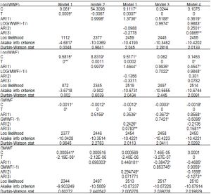	Table 4- Trend and Autoregressive models without structural breaks 1971:Q1 – 2010:Q3 Notes: *, **, and *** is 1%, 5% and 10% significance level. Log(WWF), Log(MWF), GWWF, and GMWF are semi-log models of first two panels for the level of woman work force, man work force, growth of woman work force, and growth of man work force.
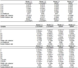	Table 5- Estimation with structural breaks, industrial production and stock market: 1971-2010 Notes: structural break points entered as a dummy variable is 1973 September (oil shock and stock market crash in the UK between 1973-75), 1987 October (black Monday crash), 1992 September (black Wednesday stock market crash), 1997 July (Asian crisis), 1998 August (Russian crisis), and 2008 September (Russian crisis and automotive industry crisis). First panel, a dummy variable of 1997 September was set to estimate step-wise structural break. Log(SP) and Log(IP) indicates stock index price, and industrial production index obtained from the IMF international financial statistics. Both SP and IP were a rolling moving averaged series with 2 month intervals. *, **, and *** is 10%, 5% and 1% significance level.
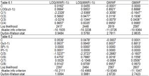	Table 6- Volatility estimation with the EGARCH model: 1971-2010 Notes: Estimator of maximum likelihood with ARCH (Marquardt) assuming normal distribution, LOG(GARCH) = C(1) + C(2)*ABS(RESID(-1)/@SQRT(GARCH(-1))) + C(3)*RESID(-1)/@SQRT(GARCH(-1)) + C(4)*LOG(GARCH(-1)) for the first panel results and LOG(GARCH) = C(5) + C(6)*ABS(RESID(-1)/@SQRT(GARCH(-1))) + C(7)*RESID(-1)/@SQRT(GARCH(-1)) + C(8)*LOG(GARCH(-1)) for the second panel results.
	Table 7- Vector Autoregression Estimates Notes: t-statistics in [ ]
	Table 8- Covariance and Correlation in level and growth of employment 1971-2010
	Table 9- Causality with 2 and 4 time lag intervals in level and growth of employment 1971-2010 Null hypothesis: column does not cause row Notes: F-statistics (at least 5% level of significance)
	Table 10- Johansen test for cointegration -number of Cointegrating Relations by Model: 1971-2010 Notes: *Critical values based on MacKinnon-Haug-Michelis (1999), Selected (0.05 level*), Notes: RMSE is Root Mean Squared Error; and MAE, Mean Absolute Error. Model 1.1 and 2.1 include their own lagged variable; Model 1.2 and 2.2 include their own lagged and each man and woman’s level of employment and their lagged variables; Model 1.3 and 2.3 include production and stock market variables in addition to all variables in Model 1.2 and 2.2. In the figures below, WWFF and MWFF are the forecasting variable of female work force and male work force respectively. The level of female work forces has narrowed standard error with more foreseeable upward direction including five year out-of-same period, actual observations used for the estimation are 474. The White heteroscedasticity consistent coefficient covariance was used in each estimation. The left-hand side column are the forecasted levels of male employment; and on the right-hand-side column are the forecasted levels of female employment.