ISSN : 0975-2927
EISSN : 0975-9166

ANIL KANNUR1*, ASHA KANNUR2*, VIJAY S RAJPUROHIT3*
1Department of Computer Science & Engineering, Shaikh College of Engineering & Technology, Belgaum, India
2Department of Electronics & Communication, Shaikh College of Engineering & Technology, Belgaum, India
3Department of Computer Science & Engineering, Gogte Institute of Technology, Belgaum, India
* Corresponding Author : vijaysr2k@yahoo.com
Received : 10-08-2011 Accepted : 06-09-2011 Published : 08-09-2011
Volume : 3 Issue : 2 Pages : 62 - 73
Int J Mach Intell 3.2 (2011):62-73
DOI : http://dx.doi.org/10.9735/0975-2927.3.2.62-73
Conflict of Interest : None declared
This paper describes a different neural network model for classification and grading of bulk seeds samples using different artificial neural network models. Algorithms are developed to acquire and process color images of bulk seeds samples. Different seeds like Groundnut, Jowar, Wheat, Rice, Metagi, Red gram, Bengal gram, and Lentils etc. are considered for the study. The developed algorithms are used to extract over 11 (9 color, area and equidiameter) features, 18 (color only) features and 20 (18 color and 2 boundary) features. The area and equidiameter features are extracted from the watershed segmentation. Different types of Neural Network based classifier is used to identify the unknown seeds samples. The classification is carried out using different types of features sets, viz., color, area and equidiameter. Classification accuracies of over 85% are obtained for all the seeds types using all the three feature sets. And also different neural network gives different accuracies and time period taken for training all the three feature sets.
Classification, Grading, Watershed, Extraction, Seeds, Neural, Elman’s, Cascade-Forward, Feed-Forward.
In the past few years, automation and intelligent sensing technologies have revolutionized our food production and processing routines. Machine vision systems (MVS) provide an alternative to manual inspection of seeds samples for kernel characteristic properties and the amount of foreign material. During seeds handling operations, information on seeds type and seeds quality is required at several stages before the next course of operation system; seeds type and quality are rapidly assessed by visual inspection. These initiatives have been accredited to the rising concerns about food quality and safety. Also, rising labor costs, shortage of skilled workers, and the need to improve production processes have all put pressure on producers and processors (Van Henten et al. 2006) [5] . In such a scenario, automation can reduce the costs by promoting production efficiency. Automated solutions, such as quality grading and monitoring (Chao et al. 2000) [9] , post-harvest product sorting (Wen and Tao 2000) [8] , and robotics for field operations (Van Henten et al. 2006) [5] . often integrate machine vision technology for sensing due to its non-destructive and accurate measurement capability (Chen et al. 2002) [10] . The information acquired using imaging sensors contains geometric, color, and texture characteristics of the objects and these physical attributes have to be extracted using image processing algorithms.
Determining the potential of morphological features to classify different seeds species, classes, varieties, damaged seeds, and an impurity, using statistical pattern recognition techniques, has been the main focus of much of the published research. Some researchers have tried to use color features for seeds identification. Only limited work has been done to incorporate textural features for classification purposes. Efforts have also been made to integrate all these features in terms of a single classification vector for seeds kernel identification. Most of the published research mainly focuses on identifying a seeds type from digital images acquired by placing kernels in a non-touching fashion. Such experiments are comparatively easier to perform in controlled situations, as in a research lab, but would be difficult to implement on site because of cumbersome setup requirements. Such systems generally require a device to present kernels in a non-touching manner, an independent conveyor belt assembly, and the typical imaging devices in order to perform the task in real-time. The algorithms for classification of seeds type used with such images are based on morphological, color, boundary features, and combination of two or more features. The pre-processing operations such as background removal, and object extraction, which are a prerequisite to determining morphological features, are some of the most time-consuming operations.
Recent research has shown that machine vision has the potential to become a viable tool to identify seeds types (Majumdar and Jayas 1999) [11] . Most of these studies have utilized well-defined images of seeds kernels acquired under controlled conditions. Under controlled situations, seeds kernels are usually placed apart from each other during image acquisition. In an industrial setup, where these systems will finally be implemented, seed kernels touch each other or even overlap. Available imaging techniques utilize two-dimensional imagery to represent original three-dimensional objects. Such two-dimensional representation poses difficulty in recognizing individual items that touch or overlap with one another in a single image. Touching and overlapping of particles renders the extraction of shape and size parameters very difficult making recognition tasks impossible. Moreover, physical separation of particles using mechanical means prior to imaging is not always practical. Therefore, implementation of machine vision in seeds handling requires availability of algorithms that could separate occluding groups of seed kernels in digital images. Refer [Fig-1.1] , for the proposed methodology for classification and grading of bulk seeds.
The training function can be any of the backprop training functions such as TRAINGD, TRAINGDM, TRAINGDA, TRAINGDX, etc… Algorithms which take large step sizes, such as TRAINLM, and TRAINRP, etc., are not recommended for Elman networks. Because of the delays in Elman networks the gradient of performance used by these algorithms is only approximated making learning difficult for large step algorithms. The learning function can be either of the backpropagation learning functions such as LEARNGD, or LEARNGDM. The performance function can be any of the differentiable performance functions such as MSE or MSEREG. Elman networks consist of Nl layers using the weight function, net input function, and the specified transfer functions. The first layer has weights coming from the input. Each subsequent layer has a weight coming from the previous layer. All layers except the last have a recurrent weight. All layers have biases. The last layer is the network output. Each layer's weights and biases are initialized with INITNW. Adaption is done with TRAINS which updates weights with the specified learning function.
The transfer functions can be any differentiable transfer function such as TANSIG, LOGSIG, or PURELIN. The training function can be any of the backprop training functions such as TRAINLM, TRAINBFG, TRAINRP, TRAINGD, etc… TRAINLM is the default training function because it is very fast, but it requires a lot of memory to run. If you get an "out-of-memory" error when training try doing one of these:
(1) Slow TRAINLM training, but reduce memory requirements, by reducing Network training Parameter by 2 or more.
(2) Use TRAINBFG, which is slower but more memory efficient than TRAINLM.
(3) Use TRAINRP which is slower but more memory efficient than TRAINBFG.
The learning function can be either of the backpropagation learning functions such as LEARNGD, or LEARNGDM. The performance function can be any of the differentiable performance functions such as MSE or MSEREG. A cascade-forward network consists of Nl layers using the weight function, net input function, and the specified transfer functions. The first layer has weights coming from the input. Each subsequent layer has weights coming from the input and all previous layers. All layers have biases. The last layer is the network output. Each layer's weights and biases are initialized with INITNW. Adaption is done with TRAINS which updates weights with the specified learning function.
The transfer functions can be any differentiable transfer function such as TANSIG, LOGSIG, or PURELIN. The training function can be any of the backprop training functions such as TRAINLM, TRAINBFG, TRAINRP, TRAINGD, etc… TRAINLM is the default training function because it is very fast, but it requires a lot of memory to run. If you get an "out-of-memory" error when training try doing one of these:
(1) Slow TRAINLM training, but reduce memory requirements, by reducing Network training Parameter by 2 or more.
(2) Use TRAINBFG, which is slower but more memory efficient than TRAINLM.
(3) Use TRAINRP which is slower but more memory efficient than TRAINBFG.
The learning function BLF can be either of the backpropagation learning functions such as LEARNGD, or LEARNGDM. The performance function can be any of the differentiable performance functions such as MSE or MSEREG. Feed-forward networks consist of Nl layers using the weight function, net input function, and the specified transfer functions. The first layer has weights coming from the input. Each subsequent layer has a weight coming from the previous layer. All layers have biases. The last layer is the network output. Each layer's weights and biases are initialized with INITNW. Adaption is done with TRAINS which updates weights with the specified learning function.
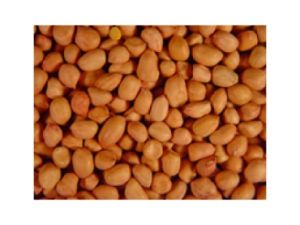
In this, RGB components are separated (see figure 3), and then the color features extracted. And two more features namely area and equidiameter are extracted using watershed segmentation as explained in section 4.2.
The extraction of RGB and HSI Color features (for the list see [Table-1.1] , [Table-1.2] , & [Table-1.3] ) is as follows:
Input: Original 24-bit color image.
Output: 18 color features.
Start
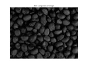
Step 1: Separate the RGB components from the original 24-bit input color image. First step in extraction of RGB features is separation of RGB components from the original color image sample [Fig-4.1a] , [Fig-4.1b] , [Fig-4.1c] .
Step 2: The Red, Green, and Blue Components of original image of a sample grain and their respective histogram are shown in [Fig-4.1d] , [Fig-4.1e] , [Fig-4.1f] . The RGB mean, variance, and range are computed using the following expressions:
…… eq. 4.1
…… eq. 4.2
…… eq. 4.3
Maximum element and minimum elements from given input image is:
max1 = max(image), max2 = max(max1)
min1 = min(image), min2 = min(min1)
The above function returns the row vector containing maximum element from each column, similarly find minimum element from whole matrix. Range is the difference between the maximum and minimum elements
Range = max2-min2 …… eq. 4.4
Step 3: Obtain the HSI components from RGB components using the equations:
.. eq. 4.5
.. eq. 4.4
.. eq. 4.4
Step 4: Find the mean, variance, and range for each RGB and HSI components using the equations 4.1, 4.3, and 4.4
Stop.
The watershed segmentation algorithm and features extraction is introduced. The features like area and equidiameter which computed using region prop function after the watershed segmentation. And also the analysis of the algorithm is done using a sample image of groundnut.
Input: 24-bit color image
Output: Segmented image and two boundary features.
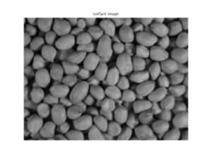
Step 1: Reading of original image which is an atomic force microscope image of a surface coating [Fig-4.2a] .
Step 2: Type Conversion: Converting the RGB image to gray color image [Fig-4.2b] .
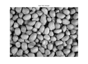
Step 3: Maximize Contrast: The top-hat transform is defined as the difference between the original image and its opening [Fig-4.2c] . The opening of an image is the collection of foreground parts of an image that fit a particular structuring element. The bottom-hat transform is defined as the difference between the closing of the original image and the original image [Fig-4.2d] .
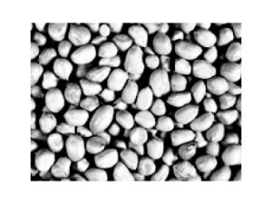
Step 4: Subtract Images: To maximize the contrast between the objects and the gaps that separate them from each other, the "bottom-hat" image is subtracted from the "original + top-hat" image [Fig-4.2e] .
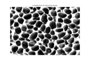
Step 5: Convert Objects of Interest: Recall that watershed transform detects intensity "valleys" in an image. We use the complement function on our enhanced image to convert our objects of interest to intensity valleys [Fig-4.2f] .
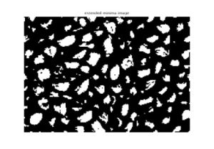
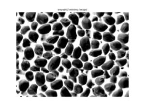
Step 6: Detect Intensity Valleys: The location [Fig-4.2g] rather than the size of the regions in the imextendedmin image is important. The imimposemin function will modify the image to contain only those valleys found by the imextendedmin function. The imimposemin function will also change a valley's pixel values to zero [Fig-4.2h] .
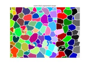
Step 7: Watershed Segmentation: Watershed segmentation of the imposed minima image is accomplished with the watershed function [Fig-4.2i] .
Step 8: Extract Features from Label Matrix.
The Neural Network is designed and implemented using the MATLAB 6p5 with Neural Network Toolbox 4.0. Jayas et al. (2000). There are four steps in the training process:
(i) Assemble the training data
(ii) Create the network.
(iii) Train the network.
(iv) Test and validate network response to new inputs.
The number of nodes in the hidden layer is calculated using the formula:
…… eq. 5.1
Where n=number of nodes in hidden layer,
I=number of input nodes (features),
O=number of output nodes, and
y=number of input patterns in the training set
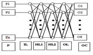
For all types of Neural Network a common model is used, which consists of four layers with eight nodes at the output layer and number of nodes in input layer depend on the number of features used (See [Fig-5.1] ). In this study, we have used three different sets of features (11, 18, & 20 Features). For all training images, color and boundary features are extracted and stored in the databases.
Input: Initial network with random weights.
Output: Update network with weights modified according to training patterns which are used for testing new samples for classification.
Start Step 1: Initialize the weights in the network (randomly).
Step 2: repeat
For each example e in the training set do
Forward pass
O=actual neural net out-put for e; T= desired output (target) for e; Calculate error (T-O) at the output
Backward pass
Compute delta_wi (changes in weight) for all weights from hidden layer to output layer;
Compute delta_wi for all weights from input layer to hidden layer;
Update the weights in the network;
End Until all examples classified correctly or stopping criterion satisfied
Return (network).
Stop
During training for identification of a grain, the ANNs are presented with binary output data. There are eight output variables representing eight grain types and two grades. For a particular grain images, its corresponding value should be one and others should be zero.
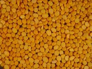
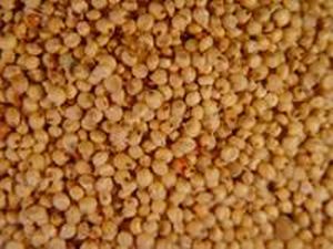
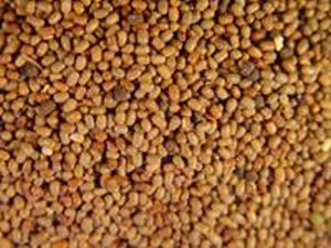
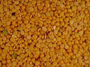
This section gives the results of exhaustive experimentation of developed methodology. A total of 480 images of seeds samples (60 of each seeds type, see figure 2.1) are used in this experiment. Different Neural Network is used for training, learning, testing, and validating the images.
Different ANN works in a different way, some of these reduce memory size and some reduces training time period. The comparison of all the networks is as shown in the figure. The Elman’s network takes more time in training the neural network for the features sets mentioned in this study. So Elman’s network is not feasible to use compared to others. Next is Cascade-Forward network is better than Elman’s network. The Cascade-Forward network takes more in training but reduces the memory size. Among the different ANN, the better one is Feed-Forward network, which trains neural network fast and takes less memory compared to Elman’s network. The performance (blue line in [Fig-6.1] ) of all three neural networks is as shown in the [Fig-6.1] , the feed-forward network reaches goal (black line in [Fig-6.1] ) within 20-30 iterations whereas the other two networks cascade-forward and Elman’s network requires more than 1000 iterations to reach the goal for the same set of features.
The feature set used consists of 9 color features and 2 boundary features for the analysis. The 9 color features are mean, variance & range of RGB components and 2 boundary features are area and equi-diameter. A four layer Neural Network is used to develop a classifier. It consists of 11 input nodes, 12 nodes in each of the two hidden layers, and 8 output nodes, one for each grain type (11-18-18-8 neural network).
The feature set used consists of 18 color features for the analysis. The 18 color features are mean, variance & range of RGB and HSI components. A four layer Neural Network is used to develop a classifier. It consists of 18 input nodes, 12 nodes in each of the two hidden layers, and 8 output nodes, one for each grain type (18-19-19-8 neural network).
The feature set used consists of 18 color features and 2 boundary features for the analysis. The 18 color features are mean, variance & range of RGB and HSI components and 2 boundary features are area and equi-diameter. A four layer Neural Network is used to develop a classifier. It consists of 20 input nodes, 12 nodes in each of the two hidden layers, and 8 output nodes, one for each grain type (20-20-20-8 neural network).
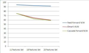
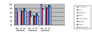
The summarized results shown in [Fig-6.2] and [Fig-6.3] , the classification accuracy, as expected, is very high for all the seeds types. In this study, the three different types of ANN models are developed and tested, the better result is given by Feed-forward network and other types are very slow in training. The performance of the feed-forward network is good for the study and for other applications as it takes less time in training and uses less memory space.
The maximum and minimum grain classification accuracy is found to be 100% and 85% respectively. The results from this study can be used for rapid identification of grain types when they arrive in railcars at the terminal grain elevators. The work carried out has relevance to real world classification of seeds and it involves both image processing and pattern recognition techniques. The watershed segmentation is used for more accuracy in classifying different types of seeds. The images in this study are acquired from clean seeds samples. For future study, the effect of percentage of foreign material on classification accuracy can be investigated using images of bulk samples and separation of seeds using images of touched seeds. Among the different ANN, the Feed-forward network is better to use for this kind of study.
[1] Cyril Voyant, Marc Muselli, Christophe Paoli, Marie-Laure Nivet (2010) CNRS, Corte.
» CrossRef » Google Scholar » PubMed » DOAJ » CAS » Scopus
[2] Jayanta Kumar Basu, Debnath Bhattacharyya, Tai-hoon Kim (2010) IJSEA Vol. 4, No. 2.
» CrossRef » Google Scholar » PubMed » DOAJ » CAS » Scopus
[3] Rojalina Priyadarshini, Nillamadhab Dash, Tripti Swarnkar, Rachita Misra (2010) Special Issue of IJCCT Vol.1 Issue 4.
» CrossRef » Google Scholar » PubMed » DOAJ » CAS » Scopus
[4] Frauke Günther and Stefan Fritsch (2010) The R Journal Vol. 2/1.
» CrossRef » Google Scholar » PubMed » DOAJ » CAS » Scopus
[5] Van Henten E.J., Van Tuiji B.A.J., Hoogakker G.J., Van Der Weerd M.J. (2006) Biosystems Engineering, 94.
» CrossRef » Google Scholar » PubMed » DOAJ » CAS » Scopus
[6] Zhang M., Laszlo L. Mark M., Krutz G. and Cyrille (1999) The International Society for Optical engineering, vol. 3543, 208-219.
» CrossRef » Google Scholar » PubMed » DOAJ » CAS » Scopus
[7] Wang W. and Paliwal J. (2004) North central CSAE/ASAE Conference Canada.
» CrossRef » Google Scholar » PubMed » DOAJ » CAS » Scopus
[8] Wen Z. and Tao Y. (2000) Transactions of the ASAE, 43(2); 449-452.
» CrossRef » Google Scholar » PubMed » DOAJ » CAS » Scopus
[9] Chao K.P., Su Y.C., Chen C.S. (2000) J. Appl. Phycol. 12, 53–62.
» CrossRef » Google Scholar » PubMed » DOAJ » CAS » Scopus
[10] Chen J. et al. (2002) Proc. Natl Acad. Sci. USA, 99, 12257–12262.
» CrossRef » Google Scholar » PubMed » DOAJ » CAS » Scopus
[11] Majumdar S. and Jayas D.S. (1999) Journal of Agricultural Engineering Research. 73 (1): 35-47.
» CrossRef » Google Scholar » PubMed » DOAJ » CAS » Scopus
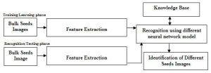 | Fig. 1.1- Proposed methodology block diagram |
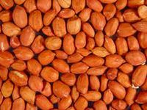 | Fig. 2.1a- Groundnut Image of Bulk Seeds Samples used in this study |
 | Fig. 2.1b- Redgram Image of Bulk Seeds Samples used in this study |
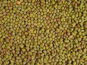 | Fig. 2.1c- Greengram Image of Bulk Seeds Samples used in this study |
 | Fig. 2.1d- Jowar Image of Bulk Seeds Samples used in this study |
 | Fig. 2.1e- Metagi Image of Bulk Seeds Samples used in this study |
 | Fig. 2.1f- Bengalgram Image of Bulk Seeds Samples used in this study |
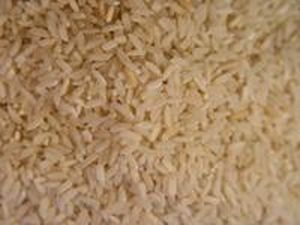 | Fig. 2.1g- Rice Image of Bulk Seeds Samples used in this study |
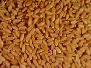 | Fig. 2.1h- Wheat Image of Bulk Seeds Samples used in this study |
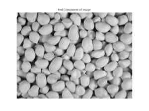 | Fig. 4.1a- Red Component of sample – RGB Components and their Histograms Images separated using Algorithm 1 |
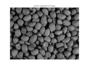 | Fig. 4.1b- Green Component of sample – RGB Components and their Histograms Images separated using Algorithm 1 |
 | Fig. 4.1c- Green Component of sample – RGB Components and their Histograms Images separated using Algorithm 1 |
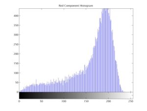 | Fig. 4.1d- Red Component Histogram of sample – RGB Components and their Histograms Images separated using Algorithm 1 |
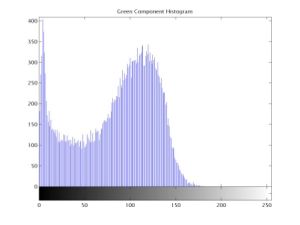 | Fig. 4.1e- Green Component Histogram of sample – RGB Components and their Histograms Images separated using Algorithm 1 |
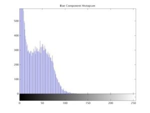 | Fig. 4.1f- Green Component Histogram of sample – RGB Components and their Histograms Images separated using Algorithm 1 |
 | Fig. 4.2a- Original Image – Images generated by Watershed Segmentation for extracting boundary features using Algorithm 2 |
 | Fig. 4.2b- Surface Image – Images generated by Watershed Segmentation for extracting boundary features using Algorithm 2 |
 | Fig. 4.2c- Top-Hat Image – Images generated by Watershed Segmentation for extracting boundary features using Algorithm 2 |
 | Fig. 4.2d- Bottom - Hat Image – Images generated by Watershed Segmentation for extracting boundary features using Algorithm 2 |
 | Fig. 4.2e- Subtract Image – Images generated by Watershed Segmentation for extracting boundary features using Algorithm 2 |
 | Fig. 4.2f- Binary Image – Images generated by Watershed Segmentation for extracting boundary features using Algorithm 2 |
 | Fig. 4.2g- Imposed Image – Images generated by Watershed Segmentation for extracting boundary features using Algorithm 2 |
 | Fig. 4.2h- Watershed Image – Images generated by Watershed Segmentation for extracting boundary features using Algorithm 2 |
 | Fig. 5.1– An Artificial Neural Network Model block diagram |
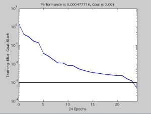 | Fig. 6.1a- Feed-Forward Performance after 24 iterations – Performance of three Artificial Neural Networks |
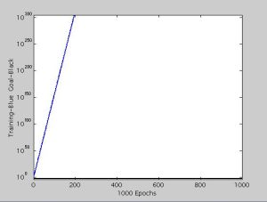 | Fig. 6.1b- Elman’s Network Performance after 1000 iterations – Performance of three Artificial Neural Networks |
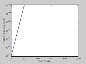 | Fig. 6.1c- Cascade-Forward Network Performance after 1000 iterations – Performance of three Artificial Neural Networks |
 | Fig. 6.2– Performance Comparisons of three Neural Network Models (blue line – Feed-forward, red line – Elman’s N/W, green line – Cascade Forward N/W) |
 | Fig. 6.3– Comparisons of three Features sets in classification & grading |
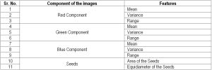 | Table 1.1– Eleven Features set consisting of RGB components of images and Boundary features. |
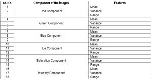 | Table 1.2– Eighteen Features set consisting of RGB components and HSI components of images |
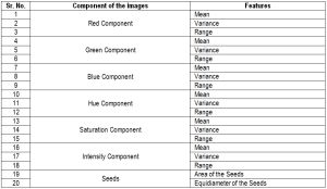 | Table 1.3– Twenty Features set consisting of RGB components, HSI components of images & Boundary features. |
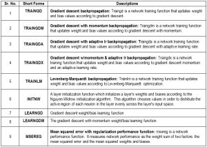 | Table 1.4- Appendix – Abbreviations used in this paper and their descriptions |