FEATURE SELECTION BY ATTRIBUTE CLUSTERING OF INFECTED RICE PLANT IMAGES

SANTANU PHADIKAR¹*, JAYA SIL², ASIT KUMAR DAS^3
1Department of Computer Science and Engineering, West Bengal University of Technology, Salt Lake, Kolkata, India
²Department of Computer Science and Technology, Bengal Engineering and Science University, Shibpur, Howrah, India
³Department of Computer Science and Technology, Bengal Engineering and Science University, Shibpur, Howrah, India
* Corresponding Author : sphadikar@yahoo.com

Received : 10-08-2011     Accepted : 05-09-2011     Published : 08-09-2011
Volume : 3     Issue : 2       Pages : 74 - 88
Int J Mach Intell 3.2 (2011):74-88
DOI : http://dx.doi.org/10.9735/0975-2927.3.2.74-88

Conflict of Interest : None declared

Automatic diagnosis of rice plant diseases at an early stage and taking corrective measures in time saves damages of rice crop across the world. The paper aims at developing an appropriate methodology to classify diseases with the help of feature sets obtained by analyzing images of infected rice plants acquired from the field. Since all features are not important in classifying diseases; selection of optimum features is a challenging task to address the problem. The work is performed in three steps. Firstly thirty six features of different category are extracted from the diseased plant images using image processing techniques. Secondly information gain (IG) of each attribute with respect to other attributes is calculated following the concept of information entropy theory. Thirdly using IG, functional dependency of the attributes are evaluated based on which fourteen significant attributes out of thirty six are selected, sufficient to classify the diseases. The proposed method has been applied on four hundred fifty infected rice plant images having three different classes. With the reduced feature set, classification accuracy is calculated using different classifiers demonstrating effectiveness of the proposed model.

Information Entropy Theory, Rice Diseases, Feature selection, Attribute Clustering, Reduct Generation.

Rice is one of the most widely cultivated food crops throughout the world. Damages due to various reasons affect productivity of rice, which can be arrested to some extent by automatic diagnosis of the diseases at an early stage. Rice ‘blast’ disease caused by the fungus Pricularia Grisea [1-3] , occurs in most of the rice fields across the glove. The damages caused by ‘blast’, depend on the degree of severity of the disease. Another critical rice disease, ‘leaf brown spot’ caused by the fungus Bypolaris Oryza [4-6] is visible throughout the rice growing season. ‘Sheath rot’ disease, caused by the fungus Sarocladium Oryza [2,4,7] usually occurs on the flag leaf sheath (boot) that encloses the panicle. The lesions first appear as oblong or irregular spots about 3/16 to 5/8 of an inch long with a gray center and a reddish-brown margin. Abundant white powdery growth of the fungus is later observed inside the affected leaf sheaths and on the surface of rotted panicles. Panicles of sheaths affected before emergence rot, turn brown or reddish brown and fail to produce any grain.
With the advancement of information technology, remote sensing techniques have been used in the field of crop management, described in [8-10] . A relation among the ground disease index and remote sensing data is established in [11] to classify the diseases. Very recently, Data mining techniques [12-14] are used to discover classification rules of rice diseases and image processing and soft computing techniques are applied to automatic diagnose the field problems, as reported in [15-16] .
Studies in the field reveal that accurate diagnosis depends on the visual properties of the plants such as change of colour, shape, orientation (textures) of the infected portion of the images. However, handling large number of features increase complexity of the system and unimportant features may lead to improper classification of diseases. One of the most important problems of the automatic diagnosis process is to identify the significant information from large volume of data using appropriate data mining techniques [17-19] . Therefore, feature selection [20-23] has become an important pre-processing step to reduce complexity in building an efficient classifier [24,25] for diagnosing the diseases.
The goal of feature selection is to avoid selecting too many or too few features than is necessary. If too few features are selected, there is a high chance that the information content in this set of features is low. On the other hand, if too many (irrelevant) features are selected, the effect of noise may overshadow the information present. Hence, a trade-off is essential that must be addressed by feature selection method. Rough set based reduct [25-27] generation methods, statistical methods [28-31] and correlation-based methods [32] contributed towards developing improved dimensionality reduction techniques. Statistical methods are generally lower in computational complexity compared to the reducts and the correlation-based methods. However, reduct generation methods are significant in reducing attributes without lose of important information, therefore, producing better classification accuracy compare to other methods.
In the proposed method, different diseased rice plant images acquired from the paddy field are used as training dataset to design the classifier. Various types of image features are extracted [33-36] using image processing techniques, which are categorized based on colours, shapes and texture. Change of colour, deviation from the actual shape and non-uniformity of the infected leaf provide important information to diagnose the diseases. However, information contained in the features is not all important. In the work following steps are executed to select features to design the classifier more accurately. (i) Information gain (IG) [12] of each attribute with respect to others is calculated based on the concept of information entropy, (ii) using IG, the IG table is formed that expresses dependency relationship between the attributes, (iii) the size of the IG table is reduced by removing the elements which don't have significant influence to classify the objects (images of infected rice plants), (iv) functional dependencies [37] of the attributes are evaluated using IG values, (v) based on functional dependency of attributes, a dependency graph is constructed [38] whose vertices and edges represent attributes and degree (in-degree / out-degree) of dependency among the attributes, respectively, (vi) the attributes are clustered [39-40] depending on the in-degree / out-degree values and elements (attributes) of each cluster are sorted in ascending / descending order, (vii) score representing significance of an attribute is calculated giving equal importance of its presence both in-degree and out-degree cluster and finally (viii) the attributes are partitioned based on their score and a single attribute from each partition is taken to generate a single attribute set consisting of optimal number of attributes of the system. In the experiment, dataset with thirty six features are prepared from the collection of four hundred fifty infected rice plant images. The proposed method reduces number of features to fourteen and used for building the classifiers. Ten-fold cross validations are carried out to compute accuracy of various classifiers. Result shows that important information about the infected leave is retained that generates accurate and complete classifier able to diagnose the diseases. The paper is organized as follows: Feature extraction procedures are discussed in first section. Next section describes the single reduct generation method using information entropy and functional dependency for feature selection. Experimental procedure and result obtained from the rice plant dataset are discussed in next section and finally, conclusions are summarized in last section.

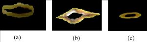
From the studies of the diseased rice plant images, it has been noticed that colour change of the infected region, shape of the spot created by the diseases and orientation (texture) of the shapes are the most important visual properties to identify the diseases. The attributes or properties are first categorized into three sub domains namely colour, shape and texture. For each sub domain, different attribute (features) values are extracted using spatial information of the image. Leave of the rice plants are infected by ‘blast’ and ‘brown spot’ diseases while stem by ‘sheath rot’ disease, described in [Fig-1] .

In order to extract features following important observations of the field experts are presented here that helps the feature extraction procedure: (i) ‘brown spots’ are dull yellow margin and dark brown center, (ii) lesions of blast create spots with a gray or white center surrounded by a reddish brown border and spots with gray center and (iii) a reddish-brown margin are created by ‘sheath rot’.
The images are first segmented using Otsu’s threshold based method [41] and then complemented to identify the background (BC) of infected region as shown in [Fig-2] . Now to separate the core (CR) and border (BR) regions of the infected images, second level segmentation is performed, respective results are shown in [Fig-3] and [Fig-4] . Colour features are obtained by calculating mean (M) and standard deviation (SD) of the intensity of pixels creating spots in three classical planes; red (R), green (G) and blue (B) of the segmented images. All 36 extracted features are listed in [Table-1] using their abbreviated name. For example, BC_M_R, and BC_SD_R represent mean and standard deviation of the spot in the background region by considering red colour plane. Similarly for border and core regions, the feature values are extracted by considering green and blue colour planes.

Area (AR), Sharpness (SH), Area-discrepancy (AD), Perimeter (PR), Eigen values (EV) and Aspect-ratio (ASR) are computed as shape based features to detecting the diseases. Here, area is determined by counting the number of pixels in the infected region while perimeter is obtained by counting the number of pixels in the boundary of the spot. These features are able to detect the variation of the shape of the spots from standard elliptical shape. Sharpness of the shape of the spot is determined by calculating the average distance between two boundary points along the major axis, labeled as T in [Fig-5] . Aspect ratio is the ratio of the major and minor axis of the ellipse that provides information regarding stretch of the spot either horizontally or vertically. The eigen value [34-35] represents valuable information, about the image of the infected region. The eigen values of the Dirichlet Laplacian [35] are preserved if the underlying domain is translated or rotated. These properties make eigen values as very useful features in recognizing shapes of different sizes and orientations. Various central moments [42] φ₁ to φ₇, invariant to scaling, translation and rotation are extracted from the infected images as shape features, as described in [Table-1] . An image moment is usually chosen to depict the global properties of the image and computed using weighted average (moment) of the intensity of pixels. Moments of all orders i.e. a complete moment set can be computed and used uniquely to describe the information contained in the image. A simple moment of a region of degree p + q is defined by equation (1), where, p and q are integers vary from 0 to 3.
m_pq = ∑ x^p y^q f(x,y) (1)
In equation(1) summation is taken over all points in the region, assuming uniform gray value in the infected region, and f(x, y) represents the brightness at a particular point (x, y). In two dimensional space, the coordinates of the centre of mass are m_x and m_y calculated by equation (2), define a unique location of the image f(x, y). It can be used as a reference point to describe the position of the image and also known as center of gravity.

; (2)

Invariance to translation is achieved by referencing all points to the center of gravity, producing the “central moments,” as described in equation (3).
µ_pq = ∑ (x-m_x)^p (y-m_y)^q f(x,y) (3)
The normalized central moments is defined as η_pq = , where, γ = . Finally, the invariant moments (φ₁ to φ₇) are computed using formulae given in [Table-2] .

Orientation of the shape is represented by the texture. Different texture features extracted from the diseased images are energy (EG), entropy (ET), contrast (CT), homogeneity (HG) and co-relation (CR), as mentioned in [Table-1] . The basic assumption of selecting EG as a feature is based on the concept that the energy distribution in frequency domain able to identify a texture. Besides providing acceptable retrieval performance from large texture database, EG based approaches are partly supported by physiological studies of the visual cortex. Another feature ET is a statistical measure of randomness and invariant to scaling, translation and rotation, used to characterize the texture of the image. It does not depend on the actual value of the gray level but only on the probabilities of gray level distribution. Local variations present in an image are measured by texture feature CT that helps to distinguish objects by their colour and brightness within the same field of view. In general, HG is defined as the quality or state of being homogeneous, used to evaluate the intensity uniformity of a local region based on high-pass operators as texture. CR measures the pixel linear dependencies of neighboring pixels, based on which uniformity in neighboring regions of image is determined. To obtain these features, colour spot images are converted to gray scale images and the co-occurrence matrix C is calculated by equation (4). Using the co-occurrence matrix the texture features [36,43] are calculated, as described in [Table-3] .
c_∆ x_∆ y (i,j)= t (4)
where,

Where f is intensity of the image of size m × n and (Δx, Δy) is the offset, considered each as one.

Once the features are extracted, the decision table is constructed with 36 features, 450 infected rice plant images and three diseases as describe in “feature extraction” section. The proposed method redefines the decision table by selecting only the relevant features, required for disease classification of infected rice plants without compromising its accuracy. The set of relevant features, called reduct [26-27,44] used to determine the optimal set of features based on the conditional entropy and functional dependency of the attributes.

Information gain is the concept applied for reducing/removing uncertainty or randomness in classifying objects with respect to some given features. Uncertainty is measured using information entropy that quantifies the expected value of information. Uncertainty relative to the given feature value is called conditional entropy contained in the features of objects. The entropy H(A) of an attribute A is defined in equation (5) and conditional entropy is referred as the entropy of A with observation of attribute B, given in equation (6).

H(A)= p(A_i) log⁡ p(A_i) (5)

(6)

Where p(A_i) is the prior probability of i^th value of A, P is the post prior probability of A_i for given B_j, j = 1, 2, .., N. The information gain IG of an attribute A with respect to another attribute B measures the reduction in uncertainty about the value of B when the value of A is known, defined as the difference between the entropy and conditional entropy values, given in equation (7).

(7)

The information gain of an attribute A with respect to attribute B (i.e.,IG ) is nothing but mutual information of A with respect to B. According to this measure, an attribute B is regarded to be more correlated to attribute A than to attribute C, if IG > IG . Since symmetry is a desired property for correlations between attributes, A and B are grouped as more likely attributes than the group consist of attributes C and B. Thus, dependency among the attributes is known using the information gain metric based on which redundancy in the datasets has been removed. For computation of information gain of attributes with respect to other attributes in a system, a decision system DS = (U, A, D) is considered, where A = {A₁, A₂, ...., A_N} is a set of N conditional attributes, U is the set of objects known as the universe of discourse and D is the decision attribute containing various class values.
The algorithm to computing information gain consists of two procedures namely, “Individual_Entropy_Computation()” and “Conditional_Entropy_Information_Gain( )”.
Algorithm: Individual_Entropy_computation (DS)
Begin
Input: DS, the decision system.
Output: Individual entropy; H(A_I) of the attribute A_I
For I = 1 to N do
{/*computation of the distinct values and their frequencies for each attribute */
Let M = No. of distinct A_I values
Let DA_I = {DA_I1, DA_I2, …………, DA_IM}/*distinct values of I^th attribute*/
INA_I = M; /* store the index value */
For J = 1 to M do
FA_{I, J} = Frequency of DA_{I, J}.
/*Compute individual entropy of each attribute using eq. (5) */
H [ A_I ] = 0; /* initialize the entropy */
For J = 1 to M do

H [ A_I ] = H [ A_I ] - log_2⁡
}
End.
Algorithm: Conditional_Entropy_Information_Gain (DS, H)
Begin
Input: Decision system DS and individual entropy H.
Output: Information gain of the system.
For I = 1 to N do /*as there are N attributes in dataset*/
{
For J = 1 to N do
{
H = 0; /* initialize the conditional entropy */
If (I ! = J) then
{
For K = 1 to | DA_I | do /*compute conditional entropy by eq. (6)
{
sum (I) = 0 ;
For L = 1 to | DA_J |
{

H = | σ_AJ = DA_JL) (σ_{AJ = DAIk} (DS)) |

/* counting frequency of distinct values in condition*/

sum(I) = sum(I) +

} /* end of L loop */
T = 0; /* initialize the total conditional entropy against each distinct value of attribute */
For L = 1 to | DA_J |

T = T- H × log₂⁡ H



} /* end of K loop */
} /* end-if */
IG(I, J)= H[ A_I ] H /*information gain by eq (7) */
} /* end of J loop */
} /* end of I loop */
End

To know the mutual information gain among attributes, equation (7) is applied for each pair of distinct attributes in the system. Thus an N×N information gain table (IG)_N×N is obtained, where the first row indicates the information gain of first attribute with respect to all attributes and so on. Each entry IG [i] [j] in the table represents the information gain value IG(i/j) obtained using equation (7). Then, for a given attribute, say in column j of IG table, average information gain is calculated and the attribute, say in row i, having greater information gain than average depends on attribute j. A functional dependency (FD) of the attributes j→ i is established and thus all N rows are checked for the dependency and set of attributes depends on attribute j are obtained. Repeating the process for j = 1, 2, ..., N, all possible mutual dependencies of the attributes are determined. Then from the functional dependencies, a dependency graph DG = (V, E) is obtained, where a directed edge V_j→V_i corresponds to functional dependency j → i. For each vertex of the graph, in-degree and out-degree parameters are evaluated where, in-degree is the number of edges incident to the vertex and out-degree is the number of edges leaves the vertex. So higher the out-degree of a vertex implies more attributes are dependent on the attribute, mapped at that vertex and so it is considered as a valuable attribute of the system. Similarly, lower the in-degree of a vertex implies it is dependent on less number of attributes, mapped at the vertices and so considered as a valuable attribute of the system. Therefore, a higher out-degree and lower in-degree is expected for an attribute in a decision system. The functional dependencies and in-degree / out-degree of the attributes are evaluated, as described by the following algorithms.
Algorithm: Functional_Dependency_of_Attributes (DS, IG)
Begin
u = 1 /*Compute functional dependencies of attributes */
For J = 1 to N do
{
sum = 0;
For I = 1 to N do
{
If (I != J)
sum = sum + IG (I,J); /* sum of column value of each attribute */
} /* end of I loop */
avg = sum / (N-1); /* average value of each attribute */
/* Compute the attribute dependency matrix FD */
For I = 1 to N do
{
If (I!= J) then
{
If (IG(I,J) > avg) then
{/* if gain of I^th attribute given J^th attribute is greater than average gain */
v = 1
FD [u] [v] = J /*calculation of functional dependency */
v + +; /* increment the column value */
FD [u] [v] = I ;
u++; /* increment the row value */
}
}
} /* end of I loop */
} /* end of J loop */
End
Algorithm: Degree_of_Dependency (DS, FD)
Begin
/*Compute in-degree, out-degree of attributes in DS from FD and store in first and second columns array deg[ ] [ ] respectively */
u = u - 1; /* u is the number of Functional dependencies */
For I = 1 to N do
{ /* compute in and out degree for each attribute*/
deg [I] [1] = deg [I] [2] = 0;
For J = 1 to u – 1 do
{ /* J^th loop compute the in and out degree of I^th attribute*/
If(FD [J] [1] = = I) then /*out-degree*/
deg [I] [1] ++;
If(FD [J] [2] = = I) /*in-degree*/
deg [I] [2] ++;
} /* end of J loop */
} /* end of I loop */
End

Attributes are partitioned into two separate clusters based on their in-degree and out-degree values, where the most important attribute has lowest in-degree and highest out-degree values. The attributes are clustered based on their in-degree values and the clusters IN_GR₁, IN_GR₂, ……., IN_GR_m are arranged in ascending order such as CLUS_in-degree = {IN_GR₁, IN_GR₂, ...., IN_GRm}. Similarly, the clusters with attributes having same out-degree are arranged in descending order based on their out-degree values, such as CLUSout-degree = {OUT_GR₁, OUT_GR₂, ...., OUT_GR_n}.
Algorithm: Partition_based_on_Out_Degree (deg)
Begin /* partition into groups w.r.t. out-degree */
CLUS_out-degree = Ø /* it is a 2-D array, each row contains one group, initially all empty*/
row = 1;
While(1)
{/ *select maximum out-degree*/
max = deg [1] [1] ;
For I = 2 to N do
{
If (max < deg [I] [1] ) then
max = deg [I] [1] ;
}
If (max = = -1) then
break; /*partitioning done, so go out of while loop */
For I = 1 to N do /* this loop compute one group of the partition*/
{
If (deg [I] [1] = = max) then
{
deg [I] [1] = -1;
CLUS_out-degree [row] = CLUS_out-degree [row] ϵ {A_I}
}
}
row = row + 1;
} /* end of while loop */
No_out_grp = row – 1; /* number of clusters in CLUS_out-degree */
End.
Algorithm: Partition_based_on_In_Degree (deg)
Begin /* partition into groups w.r.t. in-degree */
CLUS_in-degree = Ø /* it is a 2-D array, each row contains one group, initially all empty*/
row = 1;
While(1)
{
min = First non-negative value in deg [ ] [2] / *select minimum in-degree*/
For I = 1 to N do
{
If ((min > deg [I] [2] ) && (deg [I] [2] >0))
min = deg [I] [2]
}
If (min = = -1)
break; /*partitioning done, so go out of while loop*/ For I = 1 to N do /* compute one group of the partition*/
{
If (deg [I] [2] = = min) then
{
deg [I] [2] = -1;
CLUS_in-degree [row] = CLUS_in-degree [row] á´— {A_I}
}
}
row = row + 1;
} /* end of while loop */
No_in_grp = row – 1; /*no of clusters in CLUS_in-degree */
End.
Finally, a single partition of attributes is obtained from the clusters of attributes having similar in-degree and out-degree values. Let the rank functions Rf_in and Rf_out are defined on the domain sets CLUS_in-degree and CLUS_out-degree respectively to map each element of the cluster set to the index in which it belongs, as given below in equation (8) and (9).
Rf_in (x)= I_x (8)
where, x ϵ CLUS_in-degree and Ix is the index of x in CLUS_in-degree
Rf_out (x)= I_y (9)
where, y ϵ CLUS_out-degree and I_y is the index of y in CLUS_out-degree
Based on the rank of the element, score of each attribute is computed using equation (10) where for each attribute A_i in A, it’s associated groups g₁ and g₂ with respect to CLUS_in-degree and CLUS_out-degree are obtained.

(10)

Thus, equal importance is given to both the in-degree and out-degree of the attributes to measure their score value. Finally, based on scores, the attributes are partitioned as described by the algorithm below.
Algorithm:Score_of_Attributes(CLUS_out-degree, CLUS_in-degree)
Begin /* Computation of score for each attribute*/
No_out_grp = | CLUS_out-degree |
No_in_grp = | CLUS_in-degree |
For I = 1 to N do
{
/* search the rank of the group containing Ith attribute in CLUS_out-degree */
For J = 1 to No_out_grp do
{
If (A_I ϵ CLUS_out-degree [J] ) then
{
rank_out = J;
break;
}
}
/* search the rank of the group containing attribute in CLUS_in-degree */
For J = 1 to No_in_grp do
{
If (A_I ϵ CLUS_in-degree [J] ) then
{
rank_in = J;
break;
}
}
Score [I] =
} /* end of I-th loop*/
End
Algorithm: Partition_based_on_Attribute_Score(Score)
Begin /*Partition of attributes according to their score*/
CLUS = Ø /* it is a 2-D array, each row contains one cluster of attributes, initially all empty*/
row = 1;
While(1)
{ / *select minimum score*/
min = First non-negative value in array Score;
For I = 1 to N do
{
If ((min > Score [I] ) && (Score [I] > 0)) then
min = Score [I]
}
If (min = = -1) then
break; /*partitioning done, so go out of while loop */
For I = 1 to N do /* this loop compute one cluster*/
{
If (Score [I] = = min) then
{
Score [I] = -1;
CLUS [row] = CLUS [row] {A_I}
}
}
row = row + 1;
} /* end of while loop */
No_in_clstr = row – 1; /* number of clusters in CLUS */
End
Finally, the attributes are partitioned according to their scores. Then, for each partition, repeat the same process and consider a single attribute with lowest score. Combining all such attributes with lowest score from all partitions, a compact set of attributes called reduct is obtained. The proposed algorithm for partitioning of attributes and reduct formation is given below:
Algorithm: Final_Reduct_Formation (CLUS)
Begin /*Generation of reduced set of attributes*/
RED = Ø /* it is a 1-D array that contains reduct, initially empty*/
No_in_clstr = |CLUS|
For I = 1 to No_of_clstr do
{
If (CLUS [I] is an attribute) then
RED = RED CLUS [I] same procedure for CLUS [I] to compute minimum score attribute*/
DS = (U, CLUS [I] , D)
Functional_Dependency_of_Attributes(DS, IG)
Degree_of_Dependency(DS, FD)
Partition_based_on_Out_Degree(deg)
Partition_based_on_In_Degree(deg)
Score_of_Attributes(CLUS_out-degree, CLUS_in-degree)
Let score (A1) = min_score;
RED = RED {A1};
}
}
End

The proposed method is applied on a dataset generated from 450 infected rice plant images of three diseased classes (brown spot, blast and sheath rot). The dataset contains 36 features and a decision attribute with 3 different class labels. Sample datasets for different kinds of features, calculated using the methodologies described in “feature extraction” section, and given in [Table-4] , [Table-5] and [Table-6] that contain extracted colour features, shape-based features and texture features respectively. All the numeric attributes are discretized by ChiMerge [45] discretization algorithm and is described graphically in [Fig-6] .
For each pair of 36 features, information gain is calculated as shown in [Fig-7] . Functional dependencies of the attributes are shown as dependency graph, depicted in [Fig-8] .
Now, from the dependency relationship, in-degree and out-degree of each attribute (i.e., vertex of the graph) are calculated. Then the attributes are partitioned based on their in-degree/out-degree values and are stored in CLUS_in-degree and CLUS_out-degree as shown in [Table-7] and [Table-8] respectively.
The score of each attribute is calculated using [Table-7] and [Table-8] while new cluster CLUS is formed based on their score, as listed in [Table-9] , such that score of any two attributes are same in a cluster and different in different clusters. For example, score of attribute BR_M_G is (6+1)/2 = 3.5 as it is in 6^th cluster of [Table-7] and in 1st cluster of [Table-8] . Similarly, score of all attributes are computed, where BR_M_G is of lowest score. Repeat the overall process on each element in a cluster and consider the feature from each cluster with minimum score, in case of multiple minimum score, arbitrarily one attribute is selected. For example, in case of cluster 3 in [Table-9] , repeat the process with feature set {BC_M_R, CR_M_G, EV, φ₄} and ultimately attribute EV is obtained with minimum score, shown in third column of cluster 3. Finally, combining all 14 features with minimum score, a single reduct RED = {BR_M_G, φ₁, EV, CT, BR_SD_G, CR_SD_R, φ₇, ET, SH, AD, AR, BC_SD_G, BC_SD_B, BR_SD_B} is obtained.
The well known dimensionality reduction method, of attributes from 36 to 18. “Cfs Subset Eval” method Principal Component Analysis (PCA) [46] reduces number with Genetic Search [47] (CFS) selects 19 attributes and “Consistensy Subset Eval” with Rank Search (CON) [48] method finds 20 attributes out of thirty-six extracted features of the disease images. So the rate of dimensionality reduction is higher for the proposed method compare to the existing methods, shown in [Fig-9] . The method does not reduce dimension of data by losing its decision making capability, rather it provides compatible classification accuracy obtained by various classifiers when run using “weka” tool [49] where 10-fold cross-validations are carried out, as listed in [Table-10] . In [Table-10] , other dimension reduction methods like “Chi-Squared Attribute Eval”(CHI), “Classifier Subset Eval”(CLS) [50] and “Support Vector Machine Attribute Eval”(SVM) [51] are used where first fourteen ranked attributes are considered for classification, as the proposed method selects only fourteen attributes. The accuracy of classifiers show that the proposed method is at least comparable with other dimensionality reduction methods like, PCA, CFS, CON, SVM, CLS and so on.

In the paper, functional dependencies of the attributes represent the dependency graph for the attribute set. From the dependency set in-degree and out-degree of the vertices (i.e., attributes) are measured which finally helps to compute the score of the attributes. Then, attributes are partitioned according to their scores and reduct is generated. The results show significant efficiency of the proposed method. Moreover, the proposed method is envisaged on the concept of information gain, which is an established theory of measuring uncertainty and quantified the information contained in the system.

[1] Gouramanis G. D., Cahiers Options Méditerranéennes, 15(3) 61 - 68.  
» CrossRef   » Google Scholar   » PubMed   » DOAJ   » CAS   » Scopus  

[2] Damicone J., Moore B., and Fox J., (2010) Rice Diseases in Mississippi: A Guide to Identification, Mississippi State University.  
» CrossRef   » Google Scholar   » PubMed   » DOAJ   » CAS   » Scopus  

[3] Webster R. K. (2000) Rice Blast Disease Identification Guide. Davis, Dept. of Plant Pathology, University of Californi.  
» CrossRef   » Google Scholar   » PubMed   » DOAJ   » CAS   » Scopus  

[4] OU S. H., Rice Diseases. (1985) Kew Surrey, England, Commonwealth Mycological Institute. Cambrian News(Aberystwyth) Ltd, Great Britain.  
» CrossRef   » Google Scholar   » PubMed   » DOAJ   » CAS   » Scopus  

[5] Huynh N. V. and Gaur A. (2004) Omonrice 12 102-108.  
» CrossRef   » Google Scholar   » PubMed   » DOAJ   » CAS   » Scopus  

[6] Sato H., Ando I., Hirabayashi H., Tskeuchi Y., Arase S., Kihara J., Kato H., Imbe T., and Nemoto H. (2008) Breeding Science 58, 93-96.  
» CrossRef   » Google Scholar   » PubMed   » DOAJ   » CAS   » Scopus  

[7] International Rice Research Institute, Philipines, http://www.irri.org.  
» CrossRef   » Google Scholar   » PubMed   » DOAJ   » CAS   » Scopus  

[8] Pinter P. J., Hatfield Jr. J. L., Schepers J. S., Barnes E. M., Moran M. S., Daughtry C. S. T. and Upchurch D. R. (2003) Photogrammetric Engineering & Remote Sensing 69 (6), 647-664.  
» CrossRef   » Google Scholar   » PubMed   » DOAJ   » CAS   » Scopus  

[9] Khatib H. El., Hawels F., Hamdi H. & Mowelhi N. El.. (1993) IEEE Geoscience & Remote Sensing Symposium 2, 526-528.  
» CrossRef   » Google Scholar   » PubMed   » DOAJ   » CAS   » Scopus  

[10] Kobayashi T., Kanda E., Kitada K., Ishiguro K., and Torigoe Y. (2001), Phytopathology 91(3), 316-323.  
» CrossRef   » Google Scholar   » PubMed   » DOAJ   » CAS   » Scopus  

[11] Qin Z., Zhang M., Christensen T., Li W. (2003) IEEE Geoscience & Remote Sensing Symposium 4, 2215-2217.  
» CrossRef   » Google Scholar   » PubMed   » DOAJ   » CAS   » Scopus  

[12] Witten I. H., and Frank E. (2000) Data Mining: Practical Machine Learning Tools and Techniques with Java Implementations, MK.  
» CrossRef   » Google Scholar   » PubMed   » DOAJ   » CAS   » Scopus  

[13] Han J. and Kamber M. (2001) Data Mining: Concepts and Techniques, Morgan Kaufmann, San Francisco.  
» CrossRef   » Google Scholar   » PubMed   » DOAJ   » CAS   » Scopus  

[14] Mohammed T. El., Mahmoud W. and Mahmoud B. EL. (2006) The International Arab journal of Information Technology, 3 (4), 303-307.  
» CrossRef   » Google Scholar   » PubMed   » DOAJ   » CAS   » Scopus  

[15] Sanyal P., Bhattacharya U. and Bandyopadhyay S. K.. (2007) IEEE 10th International Conference on Information Technology, 85-90.  
» CrossRef   » Google Scholar   » PubMed   » DOAJ   » CAS   » Scopus  

[16] Phadikar S. and Sil J. (2008) IEEE International Conference on Information Technology, 420-423.  
» CrossRef   » Google Scholar   » PubMed   » DOAJ   » CAS   » Scopus  

[17] Jain A., Murty M., and Flynn P. (1999) ACM Comput. Surv, 31 (3) 264 – 323.  
» CrossRef   » Google Scholar   » PubMed   » DOAJ   » CAS   » Scopus  

[18] Eugenia G. G. (2008) Data Mining in Medical and Biological Research, In-Tech Publisher.  
» CrossRef   » Google Scholar   » PubMed   » DOAJ   » CAS   » Scopus  

[19] Lu W., Han J., and Ooi B.C.. (1993) Far East Workshop Geographic Information Systems, 275-289.  
» CrossRef   » Google Scholar   » PubMed   » DOAJ   » CAS   » Scopus  

[20] Raymer M. L., Punch W. F., Goodman E.D., Kuhn L. A., and Jain A. K. (2000), IEEE Transactions on Evolutionary Computation, 4(2) 164-171.  
» CrossRef   » Google Scholar   » PubMed   » DOAJ   » CAS   » Scopus  

[21] Huang C, Huang Y., Huang X., and Cercone N., (2004) Transactions on Rough Sets.  
» CrossRef   » Google Scholar   » PubMed   » DOAJ   » CAS   » Scopus  

[22] Carreira-Perpinan M. A. (1997) Technical report CS-96-09, Department of Computer Science, University of Sheffield.  
» CrossRef   » Google Scholar   » PubMed   » DOAJ   » CAS   » Scopus  

[23] Huang Y., Huang X. and Cercone N. (2004) Transactions on Rough Sets, SpringerLink Publishers, vol. 2, pp. 1-13.  
» CrossRef   » Google Scholar   » PubMed   » DOAJ   » CAS   » Scopus  

[24] Pal S. K. and Mitr S. (1999) Soft Computing, Willey, New York.  
» CrossRef   » Google Scholar   » PubMed   » DOAJ   » CAS   » Scopus  

[25] Das A. K. and Sil J. (2010) Applied Soft Computing, Elsevier, http://dx.doi.org/10.1016/j.asoc.2010.08.008.  
» CrossRef   » Google Scholar   » PubMed   » DOAJ   » CAS   » Scopus  

[26] Pawlak Z. (1982), International journal of information and computer sciences, 11, 341-356.  
» CrossRef   » Google Scholar   » PubMed   » DOAJ   » CAS   » Scopus  

[27] Pawlak Z., (1998) Cybernetics and systems, 29 661-688.  
» CrossRef   » Google Scholar   » PubMed   » DOAJ   » CAS   » Scopus  

[28] Gupta S. C. and Kapoor V. K., (1994) Fundamental of Mathematical Statistics, Sultan Chand & Sons, A.S. Printing Press, India.  
» CrossRef   » Google Scholar   » PubMed   » DOAJ   » CAS   » Scopus  

[29] Devroye L., Gyorfi L. and Lugosi G. (1996) A Probabilistic Theory of Pattern Recognition, Springer-Verlag, New York.  
» CrossRef   » Google Scholar   » PubMed   » DOAJ   » CAS   » Scopus  

[30] Devijver P. A. and Kittler J. (1982) Pattern Recognition A Statistical Approach, Prentice Hall, Englewood Cliffs, N. J.  
» CrossRef   » Google Scholar   » PubMed   » DOAJ   » CAS   » Scopus  

[31] Stephens M., Smith N.J., Donnelly P. (2001) The American Journal of Human Genetics, 68(4), 978-989.  
» CrossRef   » Google Scholar   » PubMed   » DOAJ   » CAS   » Scopus  

[32] Tiwari R. and Singh M. P. (2010) International Journal of Computer Application, 4 (8), 28-34.  
» CrossRef   » Google Scholar   » PubMed   » DOAJ   » CAS   » Scopus  

[33] Gonzalez R. C. & Richards E. W. (2007) Digital Image Processing, Pearson Education,New Delhi, India.  
» CrossRef   » Google Scholar   » PubMed   » DOAJ   » CAS   » Scopus  

[34] Pólya G., (1954) Studies in Mathematics and Mechanics Presented to Richard von Mises, Academic Press, New York, 200–207.  
» CrossRef   » Google Scholar   » PubMed   » DOAJ   » CAS   » Scopus  

[35] Courant R. and Hilbrt D., (1965) Methods of Mathematical Physics, 2nd Edition, Interscience Publishers.  
» CrossRef   » Google Scholar   » PubMed   » DOAJ   » CAS   » Scopus  

[36] Haralick R. M. (1979) Proceedings of the IEEE, 67, 786-804.  
» CrossRef   » Google Scholar   » PubMed   » DOAJ   » CAS   » Scopus  

[37] Elmasri R. and Navathe S. B. (2000), “Fundamentals of Database Systems”, third eds., Addison Wesley, ISBN 981-405330-9.  
» CrossRef   » Google Scholar   » PubMed   » DOAJ   » CAS   » Scopus  

[38] Deo N. (1995) Graph Theory with Applications to Engineering and Computer Science, Prentice-Hall of India Pvt., India.  
» CrossRef   » Google Scholar   » PubMed   » DOAJ   » CAS   » Scopus  

[39] Kaufman L. and Rousseeuw P. (1990) Finding Groups in Data: An Introduction to Cluster Analysis, Wiley.  
» CrossRef   » Google Scholar   » PubMed   » DOAJ   » CAS   » Scopus  

[40] Davies D. L. and Bouldin W. (1979) IEEE Transactions on Pattern Recognition and Machine Intelligence, 1(2) 224 – 227.  
» CrossRef   » Google Scholar   » PubMed   » DOAJ   » CAS   » Scopus  

[41] Otsu N. (1979) IEEE Transaction on Systems, Man and Cybernetics, 9, 62-66.  
» CrossRef   » Google Scholar   » PubMed   » DOAJ   » CAS   » Scopus  

[42] Hu M. K. (1962) IEEE Transactions on Information Theory, 8, 179-187.  
» CrossRef   » Google Scholar   » PubMed   » DOAJ   » CAS   » Scopus  

[43] Bharti M. H., Liu J. J., and Macgregor J. F. (2004) Chemo metrics & Intelligence Laboratory Systems, 72, 57-71.  
» CrossRef   » Google Scholar   » PubMed   » DOAJ   » CAS   » Scopus  

[44] Lin T. Y. and Carcone N. (1997) Rough Sets and Data Mining: Analysis of Imprecise Data, Kluwer Academic Publishers.  
» CrossRef   » Google Scholar   » PubMed   » DOAJ   » CAS   » Scopus  

[45] Kerber R., ChiMerge. (1992) Int'l Conf. Artificial Intelligence, AAAI-Press, 123-128.  
» CrossRef   » Google Scholar   » PubMed   » DOAJ   » CAS   » Scopus  

[46] Karhunen J., Pajunen P. and Oja E. (1998) Neurocomputing, 22:5-20, 1998.  
» CrossRef   » Google Scholar   » PubMed   » DOAJ   » CAS   » Scopus  

[47] Hall M. A. (1998) Correlation-Based Feature Selection for Machine Learning PhD thesis, Dept. of Computer Science, Univ. of Waikato, Hamilton, New Zealand.  
» CrossRef   » Google Scholar   » PubMed   » DOAJ   » CAS   » Scopus  

[48] Liu H. and Setiono R. (1996) 13th Int'l Conf. Machine Learning, pp. 319-327.  
» CrossRef   » Google Scholar   » PubMed   » DOAJ   » CAS   » Scopus  

[49] WEKA (2011) Machine Learning Software, http://www.cs.waikato.ac.nz/~ml/.  
» CrossRef   » Google Scholar   » PubMed   » DOAJ   » CAS   » Scopus  

[50] Liu. H. and Setiono R. Chi. (1995) IEEE 7th International Conference on Tools with Artificial Intelligence, 338-39.  
» CrossRef   » Google Scholar   » PubMed   » DOAJ   » CAS   » Scopus  

[51] Tou Q., Chu D., Wang J. (2008) IEEE Transaction on Neural Networks 19, 189-193.  
» CrossRef   » Google Scholar   » PubMed   » DOAJ   » CAS   » Scopus  

	Fig. 1- Rice plant Images (a) stem infected by ‘Sheath Rot’ (b) leaf infected by ‘Blast’ (c) leaf infected by ‘Brown Spot’.
	Fig. 2- Segmented Spots in Background Region
	Fig. 3- Segmented Spots in Core Region
	Fig. 4- Segmented Spots in Border Regions
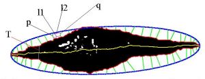	Fig. 5- Boundary of the spots corresponding to Fig. (2(b))
	Fig. 6- Decision Table of Infected Rice Images
	Fig. 7- Conditional Information Gain of the Decision Table
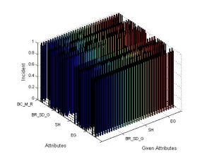	Fig. 8- 3D Plotting of Attribute Dependency Matrix
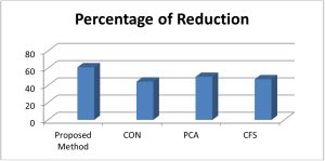	Fig. 9- Percentage of Reduction using different methods
	Table 1- Description of Features in the Dataset
	Table 2- Formulae for Normalized Central Moments
	Table 3- Generation of Texture Features
	Table 4- Sample Colour Features of the Images
	Table 5- Sample Shape Features of the Images
	Table 6- Sample Texture Features of the Images
	Table 7- Clustering Based on In-degree
	Table 8- Clustering Based on Out-degree
	Table 9- Clustering of Features Based on Scores and Final Reduct
	Table 10- Accuracy of Different Classifier for Reduced Dataset